<?xml version="1.0" encoding="utf-8"?><feed xmlns="http://www.w3.org/2005/Atom" ><generator uri="https://jekyllrb.com/" version="4.4.1">Jekyll</generator><link href="https://tanglee.top/feed.xml" rel="self" type="application/atom+xml" /><link href="https://tanglee.top/" rel="alternate" type="text/html" /><updated>2026-05-31T19:49:01+08:00</updated><id>https://tanglee.top/feed.xml</id><title type="html">Tanglee’s Blog</title><subtitle>In-progress blog site of Tanglee.
</subtitle><author><name>Tanglee</name><email>tanglili [at] iie [dot] ac [dot] cn</email></author><entry xml:lang="en"><title type="html">Fast Fourier Transform and Number Theoretic Transform</title><link href="https://tanglee.top/2026/04/29/Fast-Fourier-Transform-en.html" rel="alternate" type="text/html" title="Fast Fourier Transform and Number Theoretic Transform" /><published>2026-04-29T00:00:00+08:00</published><updated>2026-04-29T00:00:00+08:00</updated><id>https://tanglee.top/2026/04/29/Fast-Fourier-Transform-en</id><content type="html" xml:base="https://tanglee.top/2026/04/29/Fast-Fourier-Transform-en.html"><![CDATA[<p class="info"><strong>tl;dr:</strong> The Fast Fourier Transform (FFT) is generally credited to Cooley and Tukey in 1965, although its earliest ideas can be traced back to Gauss’s unpublished manuscript around 1805. FFT is one of the foundational algorithms behind modern high-performance computation: it accelerates integer multiplication and polynomial multiplication, and was named by IEEE as one of the top ten algorithms of the twentieth century. Current NIST post-quantum standards such as Kyber, Dilithium, and Falcon all involve FFT and its finite-field analogue, the Number Theoretic Transform (NTT). In addition, NTT is a critical acceleration primitive in practical zero-knowledge proof systems such as Plonk and in fully homomorphic encryption schemes such as BFV and TFHE. This article explains the mathematical theory and practical value of FFT and NTT in detail.</p>

<!--more-->

<p class="error"><strong>Disclaimer:</strong> This article is the English counterpart automatically generated from the original Chinese blog by <code class="language-plaintext highlighter-rouge">Codex</code> + <code class="language-plaintext highlighter-rouge">GPT-5</code>. The translation aims to preserve the original meaning, structure, and technical details as faithfully as possible. If there is any ambiguity or inaccuracy, please refer to the original Chinese version.</p>

<hr />

<div class="plain error" data-title="References">

  <ol>
    <li>Fast Fourier Transform, CP-Algorithms: <a href="https://cp-algorithms.com/algebra/fft.html">https://cp-algorithms.com/algebra/fft.html</a>.</li>
    <li>A note on NTT definitions and implementations: <a href="https://eprint.iacr.org/2024/585.pdf">https://eprint.iacr.org/2024/585.pdf</a>.</li>
    <li>Number Theoretic Transform, Cryptography Caffe: <a href="https://cryptographycaffe.sandboxaq.com/posts/ntt-02/">https://cryptographycaffe.sandboxaq.com/posts/ntt-02/</a>.</li>
    <li>Survey reference: <a href="https://arxiv.org/pdf/2211.13546">https://arxiv.org/pdf/2211.13546</a>.</li>
  </ol>

</div>

<h2 id="discrete-fourier-transform">Discrete Fourier Transform</h2>

<p>Let an \(n-1\) degree polynomial be written as</p>

\[A(x) = a_0 x^0 + a_1 x^1 + \dots + a_{n-1} x^{n-1}\]

<p>In particular, we assume that the polynomial degree bound, or equivalently the length of the coefficient vector, is \(n = 2^k\). In the non-power-of-two case, we can pad the higher-degree coefficients with zeros until the coefficient-vector length becomes a power of two. Let the \(n\)-th roots of unity be \(w_{n,k} = e^{\frac{2 k \pi i }{n}}\), where \(k \in [0..n-1]\), and let the primitive root of unity be \(w_{n} = w_{n, 1} = e^{\frac{2 \pi i }{n}}\). They all satisfy \(x^n = 1\).</p>

<p>The coefficient-vector representation of a polynomial is the most common one, namely \(\vec{A} = (a_0, a_1, \ldots, a_{n-1})\) above. The discrete Fourier transform is a special evaluation representation: it represents the polynomial as a vector of evaluations at the special \(n\)-th roots of unity:</p>

\[\begin{aligned}
\hat{A} &amp;= \mathsf{DFT}(\vec A) = \mathsf{DFT}(a_0, a_1, \dots, a_{n-1})\\
&amp;= (A(w_{n, 0}), A(w_{n, 1}), \dots, A(w_{n, n-1})) \\
&amp;= (A(w_n^0), A(w_n^1), \dots, A(w_n^{n-1})) \\
&amp;:= (y_0, y_1, \dots, y_{n-1}) \\
\end{aligned}\]

<p>The inverse discrete Fourier transform essentially converts the evaluation representation of a polynomial back into the usual coefficient-vector form. This transformation is also better known as Lagrange interpolation for polynomials. Thus, the (inverse) discrete Fourier transform is an algorithm for converting between these two representations, namely the following maps:</p>

\[\begin{cases}
\mathsf{DFT}_{n}: \underbrace{(a_0, a_1, \ldots, a_{n-1})}_{\text{coefficient form}} \mapsto \underbrace{(y_0, y_1, \ldots, y_{n-1})}_{\text{evaluation form}} \\
\mathsf{iDFT}_{n}: \underbrace{(y_0, y_1, \ldots, y_{n-1})}_{\text{evaluation form}} \mapsto \underbrace{(a_0, a_1, \ldots, a_{n-1})}_{\text{coefficient form}} \\
\end{cases}\]

<div class="plain error" data-title="Polynomial Multiplication via DFT">

  <p>Let \(A(x) = a_0 x^0 + a_1 x^1 + \dots + a_{n-1} x^{n-1}\) and \(B(x) = b_0 x^0 + b_1 x^1 + \dots + b_{n-1} x^{n-1}\) be arbitrary \(n-1\) degree polynomials over any ring. Then:</p>

\[\mathsf{DFT}(A(x)) \circ \mathsf{DFT}(B(x)) = \mathsf{DFT}(A(x) \cdot B(x))\]

  <p>Here \(\circ\) denotes component-wise vector multiplication, which can be computed in \(\mathcal{O}(n)\) time. If we can compute the discrete Fourier transform \(\mathsf{DFT}\) and its inverse \(\mathsf{iDFT}\) in \(\mathcal{O}(n \log n)\) time, then we can also multiply polynomials in coefficient-vector form in \(\mathcal{O}(n \log n)\) time. Let \(m \ge 2n - 1\) be the transform length. In FFT, \(m\) is usually chosen as the smallest power of two not smaller than \(2n-1\). Then:</p>

\[A(x) \cdot B(x) = \mathsf{iDFT}_{m} \left(\mathsf{DFT}_{m} \left(A\left(x\right)\right) \circ \mathsf{DFT}_{m} \left(B\left(x\right)\right)\right)\]

  <p>This is the core idea behind using the Fast Fourier Transform and the Number Theoretic Transform to accelerate polynomial multiplication and integer multiplication. In the computation above, we need to zero-pad the polynomial coefficients to length \(m\), because the final product \(A(x)\cdot B(x)\) has degree \(2(n - 1)\) and therefore has \(2n-1\) coefficients. A vector of dimension at least \(2n-1\) is needed to recover \(A(x)\cdot B(x)\) completely.</p>

</div>

<h2 id="convolution-and-fourier-transform">Convolution and Fourier Transform</h2>

<p>In communications, the Fourier transform (<strong>Continuous Time Fourier Transform</strong>) is usually a powerful tool for studying continuous signals. It converts continuous time-domain information into frequency information, or a spectrum:</p>

\[S(f) = \int_{-\infty}^{\infty} s(t) \cdot e^{-i2\pi ft} \, dt\]

<p>On existing computers, however, it is impossible to simulate a fully continuous time-domain signal. Therefore, the discrete Fourier transform has greater practical value, and this leads naturally to the discrete-time Fourier transform.</p>

<ol>
  <li>
    <p><strong>Discrete Fourier Transform (DFT)</strong> converts a sequence of complex numbers \(\{x_n\} := x_0, x_1, \dots, x_{N-1}\) into another sequence of complex numbers of the same length \(\{X_k\} := X_0, X_1, \dots, X_{N-1}\). Its forward transform is mathematically defined as follows:</p>

\[X_k = \sum_{n=0}^{N-1} x_n \cdot e^{-i 2\pi \frac{k}{N} n}, \quad k = 0, \dots, N-1\]

    <p>Here \(x_n\) is the sampled signal in the time domain, \(X_k\) is the frequency component in the frequency domain, and \(N\) is the sequence length. The term \(e^{-i 2\pi \frac{k}{N} n}\) is the complex exponential basis function, which can be expanded by Euler’s formula as \(\cos(2\pi \frac{k}{N} n) - i \sin(2\pi \frac{k}{N} n)\).</p>
  </li>
  <li>
    <p><strong>Inverse Discrete Fourier Transform (Inverse DFT)</strong> recovers the time-domain sequence from the frequency-domain sequence:</p>

\[x_n = \frac{1}{N} \sum_{k=0}^{N-1} X_k \cdot e^{i 2\pi \frac{k}{N} n}, \quad n = 0, \dots, N-1\]

    <p>Note that signal-processing conventions usually use a negative exponent for the forward DFT, whereas this article uses a positive exponent convention from the polynomial-evaluation perspective: \(y_k=\sum_{j=0}^{n-1}a_j w_n^{kj}\). The two directions are conjugate to each other; what matters is that the forward and inverse transforms are used consistently.</p>
  </li>
</ol>

<p>Switching back to the polynomial perspective, we obtain the following somewhat imprecise analogy:</p>

<table>
  <thead>
    <tr>
      <th>Time-domain representation</th>
      <th>After the discrete Fourier transform</th>
      <th>Practical meaning of the Fourier transform</th>
    </tr>
  </thead>
  <tbody>
    <tr>
      <td>Continuous time-domain signal of a wave</td>
      <td><strong>Spectrum information</strong> (frequency, amplitude, phase)</td>
      <td><strong>Frequency decomposition and component analysis of waves</strong>: decompose a superposition of waves into sinusoidal waves of single frequencies, making it easier to compute superposition and spectrum information</td>
    </tr>
    <tr>
      <td>Coefficient vector of a polynomial</td>
      <td>Evaluation form of the polynomial</td>
      <td><strong>Accelerating polynomial multiplication</strong>: by analogy with wave superposition, it enables fast convolution, i.e. multiplication</td>
    </tr>
  </tbody>
</table>

<p>In essence, <strong>convolution and multiplication are equivalent:</strong> multiplying two polynomials is essentially taking the <strong>linear convolution</strong> of their coefficient sequences. To make the later discussion of NTT more convenient, we directly consider the integer quotient ring \(\mathbb{Z}_q[x]\) here.</p>

<div class="definition" data-title="Polynomial Multiplication">

  <p>Given two \(n-1\) degree polynomials \(G(x)\) and \(H(x)\) over the commutative ring \(\mathbb{Z}_q[x]\), where \(q \in \mathbb{Z}\) and \(x\) is the polynomial variable, the multiplication of \(G(x)\) and \(H(x)\) is defined as:</p>

\[Y(x)=G(x) \cdot H(x)=\sum_{k=0}^{2(n-1)} y_k x^k\]

  <p>The new coefficient is \(y_k=\sum_{i=0}^k g_i h_{k-i} \bmod q\), where \(\boldsymbol{g}\) and \(\boldsymbol{h}\) are the coefficient vectors of the polynomials \(G(x)\) and \(H(x)\), respectively.</p>

</div>

<div class="definition" data-title="Linear Convolution">

  <p>Let \(\mathbf{g} = \{g_0, g_1, \dots, g_{n-1}\}, \mathbf{h} = \{h_0, h_1, \dots, h_{n-1}\}\) be two vectors of length \(n\). Their linear convolution \(\mathbf{y} = \mathbf{g} * \mathbf{h}\) is defined as:</p>

\[y_k = \sum_{i} g_i h_{k-i}\]

  <p>The resulting vector \(\mathbf{y}\) has length \(2n-1\), and the element index satisfies \(k \in \{0, 1, \dots, 2n-2\}\). For each \(k\), the summation range must satisfy \(0 \le i &lt; n\) and \(0 \le k-i &lt; n\).</p>

</div>

<blockquote>
  <p>It is easy to verify that the linear convolution above is equivalent to polynomial multiplication. After a polynomial is transformed into its evaluation form by the discrete Fourier transform, convolution operations become more convenient. Beyond linear convolution, cryptography often uses cyclic convolution:</p>

  <ul>
    <li>Positive wrapped convolution (PWC): equivalent to multiplication in the polynomial quotient ring \(\mathbb{Z}_q[x] / (x^n - 1)\)</li>
    <li>Negative wrapped convolution (NWC): equivalent to multiplication in the polynomial quotient ring \(\mathbb{Z}_q[x] / (x^n + 1)\)</li>
  </ul>
</blockquote>

<div class="definition" data-title="Cyclic Convolution / Positive Wrapped Convolution">

  <p>Consider two degree \(n - 1\) polynomials \(G(x)\) and \(H(x)\) in the polynomial quotient ring \(\mathbb{Z}_q[x] / (x^n - 1)\), with coefficient vectors \(\mathbf{g} = \{g_0, g_1, \dots, g_{n-1}\}, \mathbf{h} = \{h_0, h_1, \dots, h_{n-1}\}\). Their cyclic convolution \(\mathbf{y} = \mathbf{g} \circledast \mathbf{h}\) is defined by the \(k\)-th component:</p>

\[y_k = \sum_{i=0}^{n-1} g_i \cdot h_{(k-i) \pmod n} \\
\iff y_k = \sum_{i=0}^{k} g_i \cdot h_{k-i} + \sum_{i=k + 1}^{n-1} g_i \cdot h_{k + n - i}\]

  <p>where \(k \in \{0, 1, \dots, n-1\}\). The equivalent polynomial expression of this vector computation is:</p>

\[Y(x) = G(x) \cdot H(x) \pmod{x^n - 1}\]

</div>

<div class="definition" data-title="Negacyclic Convolution">

  <p>Consider two degree \(n - 1\) polynomials \(G(x)\) and \(H(x)\) in the quotient ring \(\mathbb{Z}_q[x] / (x^n + 1)\), with coefficient vectors \(\mathbf{g} = \{g_0, g_1, \dots, g_{n-1}\}, \mathbf{h} = \{h_0, h_1, \dots, h_{n-1}\}\). Their negacyclic convolution \(\mathbf{y} = \mathbf{g} \star \mathbf{h}\) is defined by the \(k\)-th component:</p>

\[y_k = \left( \sum_{i=0}^{k} g_i h_{k-i} - \sum_{i=k+1}^{n-1} g_i h_{k+n-i} \right)\]

  <p>where \(k \in \{0, 1, \dots, n-1\}\). The equivalent polynomial expression of this vector computation is:</p>

\[Y(x) = G(x) \cdot H(x) \pmod{x^n + 1}\]

</div>

<blockquote>
  <p><strong>Negacyclic convolution</strong>, also often called <strong>Negative Wrapped Convolution (NWC)</strong>, is one of the core acceleration operations in lattice-based cryptography such as Kyber and Dilithium, as well as in fully homomorphic encryption.</p>
</blockquote>

<h2 id="fast-fourier-transform">Fast Fourier Transform</h2>

<p>How can we implement \(\mathcal{O}(n \log n)\) algorithms for \(\mathsf{DFT}\) and \(\mathsf{iDFT}\)? We know that ordinary point evaluation costs \(\mathcal{O}(n)\), so the naive \(\mathsf{DFT}\) has complexity \(\mathcal{O}(n^2)\). The naive Lagrange interpolation algorithm also has complexity \(\mathcal{O}(n^2)\). The core of the Fast Fourier Transform lies in the special root-of-unity basis vector used by the evaluation representation:</p>

\[\vec w = (w_{n,0}, w_{n,1}, \ldots, w_{n,n-1}) = (w_n^0, w_n^1, \ldots, w_n^{n-1})\]

<p>The central algorithmic idea is divide and conquer. We know that:</p>

\[\begin{aligned}
A(x) &amp;= a_0 x^0 + a_1 x^1 + \dots + a_{n-1} x^{n-1} \\
&amp;= a_0 x^0 + a_2 x^2 + \dots + a_{n-2} x^{n-2} +  x(a_1 x^0 + a_3 x^2 + \dots + a_{n-1}x^{n-2}) \\
&amp;= A_0(x^2) + xA_1(x^2)
\end{aligned}\]

<p>Here \(A_0(x), A_1(x)\) are both polynomials with only \(\frac{n}{2}\) coefficients, satisfying:</p>

\[\begin{aligned}
A_0(x) &amp;= a_0 x^0 + a_2 x^1 + \dots + a_{n-2} x^{\frac{n}{2}-1} \\
A_1(x) &amp;= a_1 x^0 + a_3 x^1 + \dots + a_{n-1} x^{\frac{n}{2}-1}
\end{aligned}\]

<h3 id="dft-algorithm-mathcalon-log-n">DFT Algorithm \(\mathcal{O}(n \log n)\)</h3>

<div class="plain info" data-title="Fast Discrete Fourier Transform">

  <p>Given the coefficient vector \(\vec{A} = (a_0, a_1, \ldots, a_{n-1})\) of an \(n-1\) degree polynomial, corresponding to the polynomial</p>

\[A(x) = a_0 x^0 + a_1 x^1 + \dots + a_{n-1} x^{n-1}.\]

  <p>How can we compute its values \(\left(y_0, y_1, \ldots, y_{n-1}\right)\) at the \(n\)-th roots of unity \(\vec w = (w_{n,0}, w_{n,1}, \ldots, w_{n,n-1})\) in \(\mathcal{O}(n \log n)\) time, where \(y_i = A\left(w_{n,i}\right)\)?</p>

</div>

<p>Let \(T_{\mathsf{DFT}}(n)\) denote the time complexity of computing the discrete Fourier transform of a degree-\(n\) polynomial. From the decomposition \(A(x) = A_0(x^2) + xA_1(x^2)\), if we can obtain the \(\mathsf{DFT}\) vector of \(A\) in \(O(n)\) time from the known \(\mathsf{DFT}\) vectors of \(A_0\) and \(A_1\), then the complexity satisfies the following recurrence:</p>

\[T_{\mathsf{DFT}}(n) = 2T_{\mathsf{DFT}}(\frac{n}{2}) + \mathcal{O}(n)\]

<p>By the <a href="https://en.wikipedia.org/wiki/Master_theorem_(analysis_of_algorithms)">Master theorem</a> for recurrences, the final time complexity of this recursive algorithm is \(\mathcal{O}(n \log n)\). A key observation is that squaring the vector of \(n\)-th roots of unity, \(\vec w^2 = (w_n^0, w_n^2, \ldots, w_n^{2(n-1)})\), gives exactly all \(\frac{n}{2}\)-th roots of unity. Therefore, the input pattern in the evaluation representations of \(A_0(x)\) and \(A_1(x)\) matches that of \(A(x)\) precisely. More concretely, suppose we already know \(A_0(x), A_1(x)\) and their discrete Fourier transforms:</p>

\[\begin{cases}
\left(y_k^0\right)_{k=0}^{n/2-1} = \mathsf{DFT}(A_0) \\
\left(y_k^1\right)_{k=0}^{n/2-1} = \mathsf{DFT}(A_1)
\end{cases}\]

<p>Using the special properties of roots of unity:</p>

\[\begin{cases}
w_{n}^{2k} = e^{\frac{2\pi k i}{n/2}} =  w_{n/2}^{k} &amp; k \in [0, n/2 - 1] \\
w_{n}^{k + \frac{n}{2}}= - w_{n}^{k} &amp;  k \in [0, n - 1]
\end{cases}\]

<p>Therefore, the \(n\) evaluation values of \(\mathsf{DFT}(A)\) can be recovered as follows:</p>

\[\begin{cases}
y_k = A_0(w_n^{2k}) + w_n^{k} \cdot A_1(w_n^{2k}) =  y_k^0 + w_n^k y_k^1, &amp; k = 0, \ldots, \frac{n}{2} - 1. \\

y_k = A_0(w_n^{2k}) + w_n^{k} \cdot A_1(w_n^{2k}) = y_{k \bmod \frac{n}{2}}^{0} + w_n^{k} y_{k \bmod \frac{n}{2}}^{1}  &amp; k = \frac{n}{2}, \ldots, {n} - 1. \\
\end{cases}\]

<p>Written more elegantly:</p>

\[\begin{cases}
y_k &amp;= y_k^0 + w_n^k y_k^1, &amp;\quad k = 0 \dots \frac{n}{2} - 1, \\
y_{k+n/2} &amp;= y_k^0 - w_n^k y_k^1, &amp;\quad k = 0 \dots \frac{n}{2} - 1.
\end{cases}\]

<p>This formula is also called the butterfly formula. The whole recursive expression is quite elegant: using the butterfly formula, one only needs \(\mathcal{O}(n)\) time to recover the DFT of \(A\) from the DFTs of \(A_0\) and \(A_1\). In summary, we have obtained a recursive \(\mathcal{O}(n \log n)\) algorithm for the discrete Fourier transform \(\mathsf{DFT}\).</p>

<h3 id="idft-algorithm-mathcalon-log-n">iDFT Algorithm \(\mathcal{O}(n \log n)\)</h3>

<div class="plain info" data-title="Fast Inverse Discrete Fourier Transform">

  <p>Given the values \(\left(y_0, y_1, \ldots, y_{n-1}\right)\) of an \(n-1\) degree polynomial \(A(x) = a_0 x^0 + a_1 x^1 + \dots + a_{n-1} x^{n-1}\) at the \(n\)-th roots of unity \(\vec w = (w_{n,0}, w_{n,1}, \ldots, w_{n,n-1})\), where \(y_i = A\left(w_{n,i}\right)\), how can we compute its coefficient vector \(\vec{A} = (a_0, a_1, \ldots, a_{n-1})\) in \(\mathcal{O}(n \log n)\) time?</p>

</div>

<p>Simply put, this is polynomial interpolation. Lagrange interpolation can compute it in \(\mathcal{O}(n^2)\) time. Essentially, this is solving a system of linear equations:</p>

\[\underbrace{
\begin{pmatrix}
w_n^0 &amp; w_n^0 &amp; w_n^0 &amp; w_n^0 &amp; \cdots &amp; w_n^0 \\
w_n^0 &amp; w_n^1 &amp; w_n^2 &amp; w_n^3 &amp; \cdots &amp; w_n^{n-1} \\
w_n^0 &amp; w_n^2 &amp; w_n^4 &amp; w_n^6 &amp; \cdots &amp; w_n^{2(n-1)} \\
w_n^0 &amp; w_n^3 &amp; w_n^6 &amp; w_n^9 &amp; \cdots &amp; w_n^{3(n-1)} \\
\vdots &amp; \vdots &amp; \vdots &amp; \vdots &amp; \ddots &amp; \vdots \\
w_n^0 &amp; w_n^{n-1} &amp; w_n^{2(n-1)} &amp; w_n^{3(n-1)} &amp; \cdots &amp; w_n^{(n-1)(n-1)}
\end{pmatrix}
}_{\mathbf{V} \in \mathbb{C}^{n \times n}}
\begin{pmatrix}
a_0 \\ a_1 \\ a_2 \\ a_3 \\ \vdots \\ a_{n-1}
\end{pmatrix} = \begin{pmatrix}
y_0 \\ y_1 \\ y_2 \\ y_3 \\ \vdots \\ y_{n-1}
\end{pmatrix}\]

<p>Here \(\mathbf{V} \in \mathbb{C}^{n \times n}\) is the Vandermonde matrix. Its inverse is:</p>

\[\mathbf{V}^{-1} = 
\frac{1}{n}
\begin{pmatrix}
w_n^0 &amp; w_n^0 &amp; w_n^0 &amp; w_n^0 &amp; \cdots &amp; w_n^0 \\
w_n^0 &amp; w_n^{-1} &amp; w_n^{-2} &amp; w_n^{-3} &amp; \cdots &amp; w_n^{-(n-1)} \\
w_n^0 &amp; w_n^{-2} &amp; w_n^{-4} &amp; w_n^{-6} &amp; \cdots &amp; w_n^{-2(n-1)} \\
w_n^0 &amp; w_n^{-3} &amp; w_n^{-6} &amp; w_n^{-9} &amp; \cdots &amp; w_n^{-3(n-1)} \\
\vdots &amp; \vdots &amp; \vdots &amp; \vdots &amp; \ddots &amp; \vdots \\
w_n^0 &amp; w_n^{-(n-1)} &amp; w_n^{-2(n-1)} &amp; w_n^{-3(n-1)} &amp; \cdots &amp; w_n^{-(n-1)(n-1)}
\end{pmatrix} 
\\
\implies \begin{pmatrix}
a_0 \\ a_1 \\ a_2 \\ a_3 \\ \vdots \\ a_{n-1}
\end{pmatrix} = 
\mathbf{V}^{-1} 
\begin{pmatrix}
y_0 \\ y_1 \\ y_2 \\ y_3 \\ \vdots \\ y_{n-1}
\end{pmatrix}\]

<p>Therefore, the Lagrange interpolation formula in this special form is also very elegant. We can directly express \(a_{k}\) in polynomial form as:</p>

\[a_k = \frac{1}{n} \sum_{j=0}^{n-1} y_j w_n^{-k j}\]

<p>This gives us a problem almost identical to the expression \(y_k = \sum_{j=0}^{n-1} a_j w_n^{k j}\) for \(\mathsf{DFT}\). The key changes are:</p>

\[\begin{cases}
1  &amp;\implies \frac{1}{n} \\
w_n^{k j} &amp;\implies w_n^{-k j}
\end{cases}\]

<p>The recursive algorithm from the previous section applies equally well in this setting. In summary, we have obtained a recursive \(\mathcal{O}(n \log n)\) algorithm for the inverse discrete Fourier transform \(\textsf{iDFT}\).</p>

<blockquote>
  <p><strong>The core of FFT acceleration</strong>: The fundamental reason FFT is fast is the periodicity of roots of unity:</p>

\[w_{n}^{n} = 1, \quad w_{n}^{\frac{n}{2}} = -1\]

  <p>This allows many computations to be reused, which is the essence of the recursive acceleration. In the later discussion of NTT, we will further explain how to reuse computation through the periodicity of roots of unity.</p>
</blockquote>

<h2 id="fast-number-theoretic-transform">Fast Number Theoretic Transform</h2>

<p>In cryptography, we usually care about polynomials over integer rings. More specifically, we care about polynomials over the integer quotient ring \(\mathbb{Z}_{q}\), and in most cases we regard \(q\) as a prime. In this section, all multiplication operations are explained through convolution, namely the following correspondence:</p>

<table>
  <thead>
    <tr>
      <th>Linear Convolution</th>
      <th>Cyclic Convolution / Positive Wrapped Convolution</th>
      <th>Negacyclic Convolution</th>
    </tr>
  </thead>
  <tbody>
    <tr>
      <td>Multiplication in \(\mathbb{Z}_q[x]\)</td>
      <td>Multiplication in \(\mathbb{Z}_q[x] / (x^n - 1)\)</td>
      <td>Multiplication in \(\mathbb{Z}_q[x] / (x^n + 1)\)</td>
    </tr>
  </tbody>
</table>

<p>Over integer quotient rings, we need to find a root of unity with the same properties as \(e^{\frac{2\pi i}{n}}\) in the discrete Fourier transform: the primitive root of unity over \(\mathbb{Z}_{q}\) defined below.</p>

<div class="definition" data-title="Primitive n-th Root of Unity">

  <p>We call \(w\) a primitive \(n\)-th root of unity over \(\mathbb{Z}_{q}\) if and only if it satisfies:</p>

\[w^n \equiv 1 \bmod q, \text{ and } w^i \not\equiv 1 \bmod q, \forall i \in [1, n-1]\]

</div>

<h3 id="linear--positive-wrapped-convolution">Linear / Positive Wrapped Convolution</h3>

<div class="definition" data-title="Number Theoretic Transform (NTT)">

  <p>Let \(\omega\) be a primitive \(n\)-th root of unity over \(\mathbb{Z}_q\), and let \(A(x)\) be an \(n-1\) degree polynomial over \(\mathbb{Z}_q[x]\). The <strong>Number Theoretic Transform (NTT)</strong> of its coefficient vector \(\mathbf{a}\) is defined as \(\hat{\mathbf{a}} = \textsf{NTT}^{\omega}(\mathbf{a})\):</p>

\[\hat{\mathbf{a}}_j = \sum_{i=0}^{n-1} \omega^{ij} \mathbf{a}_i \pmod q, \quad j = 0, 1, 2, \dots, n-1\]

  <p>In particular, we know that \(\hat{\mathbf{a}}_j = A(\omega^j) \pmod{ q }\).</p>

</div>

<div class="definition" data-title="Inverse Number Theoretic Transform (iNTT)">

  <p>Let \(\omega\) be a primitive \(n\)-th root of unity over \(\mathbb{Z}_q\). The <strong>inverse Number Theoretic Transform (iNTT)</strong> of an \(n\)-dimensional evaluation vector \(\hat{\mathbf{a}}\) is defined as \(\mathbf{a} = \textsf{iNTT}^{\omega}(\hat{\mathbf{a}})\):</p>

\[\mathbf{a}_j = \frac{1}{n} \sum_{i=0}^{n-1} \omega^{-ij} \hat{\mathbf{a}}_i \pmod q, \quad j = 0, 1, 2, \dots, n-1\]

</div>

<p>It is easy to verify that the two matrices corresponding to the expressions above in \(\hat{\mathbf{a}}\) and \({\mathbf{a}}\) are inverses of each other:</p>

\[\mathbf{a} = \textsf{iNTT}^{\omega}\left(\textsf{NTT}^{\omega}\left(\mathbf{a}\right)\right)\]

<p>Thus, linear convolution can be computed via NTT as follows. Note that when computing linear convolution in \(\mathbb{Z}_q[x]\), one should choose a transform length \(m \ge 2n-1\) and zero-pad the input:</p>

\[\mathbf{c} = \mathbf{a} * \mathbf{b} = \textsf{iNTT}^{\omega}\left(\textsf{NTT}^{\omega}\left(\mathbf{a}\right) \circ \textsf{NTT}^{\omega}\left(\mathbf{b}\right)\right)\]

<p>The acceleration techniques from FFT can be transferred completely to NTT and iNTT. Earlier, we mentioned that if we want to compute linear convolution over \(\mathbb{Z}_q[x]\), the dimension of \(\mathbf{c}\) should be \(2n - 1\). <strong>If we only use an \(n\)-th primitive root of unity and a transform of length \(n\), then we do not obtain linear convolution, but cyclic convolution.</strong> At this point, switching to the polynomial perspective, the values obtained after convolution are still the genuine values of \(A(\omega^i) \cdot B(\omega^i) \bmod q\), but the coefficients of monomials of degree \(\ge n\) have been cyclically accumulated into lower-degree coefficients. Because we are using an \(n\)-th primitive root, it satisfies \(x^{n + k} = x^k\), which is equivalent to:</p>

\[x^{n+k} \equiv x^k \pmod {x^{n} - 1}\]

<p>That is, the result is reduced modulo the polynomial \({x^{n} - 1}\). In coefficient terms, the true higher-degree monomial coefficients are cyclically accumulated into lower-degree monomial coefficients, which is exactly the expression for positive wrapped convolution:</p>

\[y_k = \sum_{i=0}^{k} g_i \cdot h_{k-i} + \sum_{i=k + 1}^{n-1} g_i \cdot h_{k + n - i}\]

<p>Let \(\textsf{NTT}_{n}^{\omega}(\cdot)\) denote the number theoretic transform acting on an \(n\)-dimensional vector using the primitive generator \(\omega\). Unless otherwise specified, we omit the parameter \(n\) and assume it matches the actual vector dimension, writing it simply as \(\textsf{NTT}^{\omega}(\cdot)\). We then obtain the following proposition.</p>

<div class="proposition" data-title="NTT-based Positive Wrapped Convolution">

  <p>Let \(\mathbf{a}, \mathbf{b}\) be two \(n\)-dimensional vectors over \(\mathbb{Z}_q\), corresponding to two degree \(n-1\) polynomials, and let \(\omega\) be a primitive \(n\)-th root of unity over \(\mathbb{Z}_q\). Their positive wrapped convolution can be computed by the following number theoretic transforms:</p>

\[\mathbf{c} = \mathbf{a} \circledast \mathbf{b} = \textsf{iNTT}^{\omega}\left(\textsf{NTT}^{\omega}\left(\mathbf{a}\right) \circ \textsf{NTT}^{\omega}\left(\mathbf{b}\right)\right)\]

</div>

<p>The more essential point is that the \(n\)-th primitive roots selected by NTT all satisfy:</p>

\[x^n = 1 \iff x^n - 1= 0\]

<p>Therefore, the final result is plainly equivalent to the result after reducing modulo the polynomial \(x^n - 1\). This gives a more intuitive understanding of PWC and also helps us understand the mathematical intuition behind NWC in the next section.</p>

<h3 id="negacyclic-convolution">Negacyclic Convolution</h3>

<p>Next, consider how to compute negacyclic convolution. From the expression</p>

\[y_k = \sum_{i=0}^{k} g_i \cdot h_{k-i} - \sum_{i=k + 1}^{n-1} g_i \cdot h_{k + n - i}\]

<p>We naturally think that coefficients of monomials of degree \(\ge n\) are also accumulated into the corresponding lower-degree terms after reducing degrees modulo \(n\), except that their contribution to the coefficients is negative. Thus, we naturally want the relation \(x^{n + k} = -x^{k}\). In other words, the primitive root \(\varphi\) for this NTT should satisfy \(\varphi^{n} = - 1\), so \(\varphi\) is a primitive \(2n\)-th root of unity. However, if we simply replace \(\omega\) in positive wrapped convolution by \(\varphi\), this does not directly produce negacyclic convolution; instead, it introduces a <strong>frequency shift</strong> or a <strong>mathematical mismatch</strong>. Moreover, the evolution of twiddle factors in the standard NTT is based on the primitive-root sequence \(\omega^0, \omega^1, \omega^2, \ldots, \omega^{n-1}\) satisfying \(x^n = 1\). If we simply replace it by \(\varphi^0, \varphi^1, \varphi^2, \ldots, \varphi^{n-1}\), then half of these \(2n\)-th roots of unity do not have a consistent identity of either \(x^n = 1\) or \(x^n = -1\), and this property is crucial for fast NTT. Here I give two mathematical ways to understand NWC constructions.</p>

<p>Let \(\varphi\) be a primitive \(2n\)-th root of unity, and let \(\omega\) be a primitive \(n\)-th root of unity satisfying \(\omega = \varphi^2\).</p>

<div class="plain error" data-title="Understanding NWC Construction: View 1">

  <p>From the sequence perspective, what we need are exactly all roots satisfying \(x^n = -1\). There are exactly \(n\) such roots, and one can verify that they are precisely the following sequence:</p>

\[\{\varphi^1, \varphi^3, \varphi^5, \ldots, \varphi^{2n-1}\}\]

  <p>In other words, the roots of \(x^n+1\) are exactly the odd powers of the \(2n\)-th roots of unity. Therefore, the NTT construction based on \(\varphi\) is:</p>

\[\hat{\mathbf{a}}_j = \sum_{i=0}^{n-1} \varphi^{i(2j+1)} a_i \pmod q, \quad j = 0, 1, 2, \dots, n-1\]

</div>

<div class="plain error" data-title="Understanding NWC Construction: View 2">

  <p>Now our idea is to convert NWC into PWC, so that we can use the standard NTT defined earlier. To achieve this, we need to transform the coefficients. Define a new polynomial \(\hat{A}(y)\) by setting \(x = \varphi \cdot y\). When \(x^n = -1\), we have \((\varphi y)^n = -1 \Rightarrow \varphi^n y^n = -1\). Since \(\varphi^n = -1\), this becomes \(-y^n = -1 \Rightarrow y^n = 1\). Therefore, applying the PWC-style NTT to \(\hat{A}(y)\) gives the negacyclic NTT of the original polynomial.</p>

  <p>On coefficients, this mapping is \(\mathbf{a}'_i = \mathbf{a}_i \cdot \varphi^i\). Construct the polynomial \(A'(x) = \sum \mathbf{a}'_i x^i\) and apply the PWC-style NTT to it:</p>

\[\begin{aligned}
\hat{\mathbf{a}}_j &amp;= \sum_{i=0}^{n-1} \omega^{ij} \mathbf{a}'_i \pmod q \\
&amp;= \sum_{i=0}^{n-1}  \omega^{ij} \varphi^i \mathbf{a}_i \pmod q \\
&amp;= \sum_{i=0}^{n-1} \varphi^{i(2j + 1)} \mathbf{a}_i \pmod q
\end{aligned}\]

  <p>where \(j = 0, 1, 2, \dots, n-1\).</p>

</div>

<p>The two viewpoints above yield the same result. We obtain the formal definition of the negacyclic Number Theoretic Transform as follows.</p>

<div class="definition" data-title="Negacyclic Number Theoretic Transform">

  <p>Let \(\varphi\) be a primitive \(2n\)-th root of unity over \(\mathbb{Z}_q\). Then \(\omega := \varphi^2\) is a primitive \(n\)-th root of unity over \(\mathbb{Z}_q\). Let \(A(x)\) be an \(n-1\) degree polynomial over \(\mathbb{Z}_q[x]\). The number theoretic transform of its coefficient vector \(\mathbf{a}\) based on \(\varphi\) is defined as \(\hat{\mathbf{a}} = \textsf{NTT}^{\varphi}(\mathbf{a})\):</p>

\[\hat{\mathbf{a}}_j = \sum_{i=0}^{n-1} \varphi^i \omega^{ij} \mathbf{a}_i \pmod q, \quad j = 0, 1, 2, \dots, n-1\]

  <p>Substituting \(\omega := \varphi^2\), this is equivalent to:</p>

\[\hat{\mathbf{a}}_j = \sum_{i=0}^{n-1} \varphi^{i(2j + 1)} \mathbf{a}_i \pmod q\]

</div>

<blockquote>
  <p>Similarly, by inverting the Vandermonde matrix, we can obtain the formula for the inverse negacyclic Number Theoretic Transform. It is worth pointing out that the paper <a href="https://eprint.iacr.org/2024/585.pdf">https://eprint.iacr.org/2024/585.pdf</a> contains a major typo in its definition of iNTT.</p>
</blockquote>

<div class="definition" data-title="Inverse Negacyclic Number Theoretic Transform">

  <p>Let \(\varphi\) be a primitive \(2n\)-th root of unity over \(\mathbb{Z}_q\), and let \(\omega := \varphi^2\) be a primitive \(n\)-th root of unity over \(\mathbb{Z}_q\). The inverse number theoretic transform based on \(\varphi\) of an \(n\)-dimensional evaluation vector \(\hat{\mathbf{a}}\) is defined as \(\mathbf{a} = \textsf{iNTT}^\varphi(\hat{\mathbf{a}})\):</p>

\[\mathbf{a}_j = \frac{1}{n} \sum_{i=0}^{n-1} \varphi^{-j} \omega^{-ij} \hat{\mathbf{a}}_i \pmod q, \quad j = 0, 1, 2, \dots, n-1\]

  <p>Substituting \(\omega := \varphi^2\), this is equivalent to:</p>

\[\mathbf{a}_j = \frac{1}{n} \sum_{i=0}^{n-1} \varphi^{-j(2i + 1)} \hat{\mathbf{a}}_i \pmod q\]

</div>

<p>It is easy to verify that the two matrices corresponding to the expressions above in \(\hat{\mathbf{a}}\) and \({\mathbf{a}}\) are inverses of each other:</p>

\[\mathbf{a} = \textsf{iNTT}^\varphi \left(\textsf{NTT}^\varphi\left(\mathbf{a}\right)\right)\]

<div class="proposition" data-title="NTT-based Negative Wrapped Convolution">

  <p>Let \(\mathbf{a}, \mathbf{b}\) be two \(n\)-dimensional vectors over \(\mathbb{Z}_q\), corresponding to two degree \(n-1\) polynomials, and let \(\varphi\) be a primitive \(2n\)-th root of unity over \(\mathbb{Z}_q\). Their negacyclic convolution can be computed by the following number theoretic transforms:</p>

\[\mathbf{c} = \mathbf{a} \star \mathbf{b} = \textsf{iNTT}^{\varphi}\left(\textsf{NTT}^{\varphi}\left(\mathbf{a}\right) \circ \textsf{NTT}^{\varphi}\left(\mathbf{b}\right)\right)\]

</div>

<h3 id="the-essence-of-the-number-theoretic-transform">The Essence of the Number Theoretic Transform</h3>

<p>Returning to the algebraic perspective, the essence of the Number Theoretic Transform is ring decomposition and isomorphism. We take NWC as an example. Let \(\varphi\) be a primitive \(2n\)-th root of unity over \(\mathbb{Z}_q\). Then the cyclotomic polynomial \(C(X) = X^{n} + 1\) has the following factorization:</p>

\[C(X) = \prod_{i=0}^{n-1} (X - \varphi^{2i + 1})\]

<p>By the Chinese Remainder Theorem, there is a ring isomorphism:</p>

\[\mathbb{Z}_q[X] / (X^n + 1) \cong \prod_{i=0}^{n-1} \mathbb{Z}_q[X] / (X - \varphi^{2i + 1})\]

<p>For each factor \(\alpha = \varphi^{2i + 1}\), we have \(\mathbb{Z}_q[X] / (X - \alpha) \cong \mathbb{Z}_q\) through the map \(X \mapsto \alpha\), i.e. evaluating the polynomial at the point \(\alpha\). Therefore, the isomorphism above can be further simplified as:</p>

\[\mathbb{Z}_q[X] / (X^n + 1) \cong \underbrace{\mathbb{Z}_q \times \mathbb{Z}_q \times \dots \times \mathbb{Z}_q}_{n} \cong \mathbb{Z}_q^n\]

<p>For a polynomial \(A(X) \in \mathbb{Z}_q[X] / (X^n + 1)\) with coefficient vector \(\mathbf{a}\), the NTT and inverse NTT are essentially a ring isomorphism.</p>

\[\begin{aligned}
\textsf{NTT}: 
\mathbb{Z}_q[X] / (X^n + 1) \mapsto \mathbb{Z}_q^{n} &amp;\implies
\mathbf{a} \mapsto (A(\varphi^{1}), A(\varphi^{3}), \dots, A(\varphi^{2n-1}))\\
\textsf{iNTT}: 
\mathbb{Z}_q^{n} \mapsto \mathbb{Z}_q[X] / (X^n + 1) &amp;\implies
(A(\varphi^{1}), A(\varphi^{3}), \dots, A(\varphi^{2n-1})) \mapsto \mathbf{a} \\
\end{aligned}\]

<p>The essence of the Fast Fourier Transform and the fast Number Theoretic Transform is that the group isomorphism above also admits the following recursive divide-and-conquer decomposition:</p>

\[\begin{aligned}
\mathbb{Z}_q[X] / (X^n + 1) &amp; \cong  \mathbb{Z}_q[X] / (X^{\frac{n}{2}} - \varphi^{\frac{n}{2}}) \times  \mathbb{Z}_q[X] / (X^{\frac{n}{2}} + \varphi^{\frac{n}{2}})  \\
&amp;\cong  \mathbb{Z}_q[X] / (X^{\frac{n}{4}} - \varphi^{\frac{n}{4}}) \times \mathbb{Z}_q[X] / (X^{\frac{n}{4}} + \varphi^{\frac{n}{4}}) \\

&amp;\quad \times \mathbb{Z}_q[X] / (X^{\frac{n}{4}} - \varphi^{\frac{3n}{4}}) \times \mathbb{Z}_q[X] / (X^{\frac{n}{4}} + \varphi^{\frac{3n}{4}}) \\
&amp; \cong \cdots \\
&amp; \cong \prod_{i=0}^{n-1} \mathbb{Z}_q[X] / (X - \varphi^{2i + 1})
\end{aligned}\]

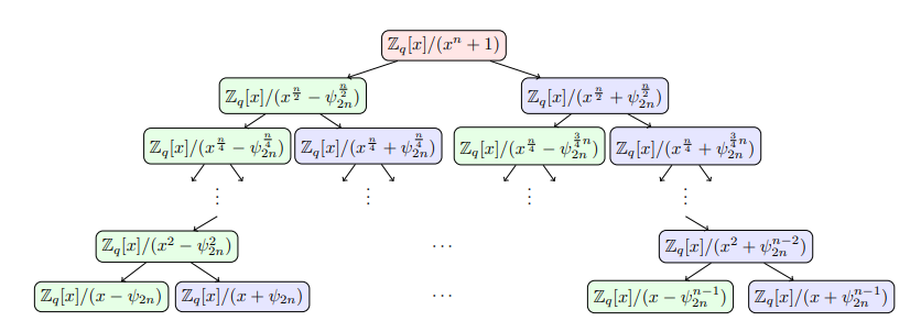
<p>That is the following CRT isomorphism map:</p>

<figure class="image-figure align-center"><img src="/assets/images/260429-fast-fourier-transform/nwc-crt-decomposition.png" alt="CRT decomposition diagram for NWC" style="width: 85%;" loading="lazy" /><figcaption>Figure 1. Recursive CRT decomposition in the NWC setting, source: https://arxiv.org/pdf/2211.13546</figcaption></figure>

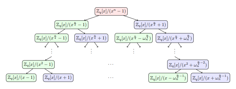
<p>Similarly, for PWC, the modulus polynomial \(x^n - 1\) admits a similar CRT isomorphism map:</p>

<figure class="image-figure align-center"><img src="/assets/images/260429-fast-fourier-transform/pwc-crt-decomposition.png" alt="CRT decomposition diagram for PWC" style="width: 85%;" loading="lazy" /><figcaption>Figure 2. Recursive CRT decomposition in the PWC setting, source: https://arxiv.org/pdf/2211.13546</figcaption></figure>

<p>From the ring-isomorphism decomposition above, we can already see the rough shape of the butterfly operation. In the next section, we introduce the butterfly operation of the fast Number Theoretic Transform, namely the Cooley-Tukey algorithm, and the butterfly operation of the fast inverse Number Theoretic Transform, namely the Gentleman-Sande algorithm.</p>

<h2 id="ctgs-butterfly-algorithms">CT/GS Butterfly Algorithms</h2>

<p>Let \(\varphi\) be a primitive \(2n\)-th root of unity over \(\mathbb{Z}_q\), and let \(\omega := \varphi^2\) be a primitive \(n\)-th root of unity over \(\mathbb{Z}_q\). Here \(n\) is exactly a power of two, so the recursion can proceed completely.</p>

<p>The key properties of the fast Fourier transform are:</p>

\[\varphi^{k+2n} = \varphi^{k} \\
\varphi^{k+n} = -\varphi^{k}\]

<p>To unify notation, let the number theoretic transform for positive wrapped convolution be denoted by \(\textsf{NTT}^{+}\), and the number theoretic transform for negacyclic convolution be denoted by \(\textsf{NTT}^{-}\). Since \(\omega := \varphi^2\), both can be written uniformly in terms of \(\varphi\):</p>

\[\begin{cases}
\textsf{NTT}^{+}: &amp; \hat{\mathbf{a}}_j = \sum_{i=0}^{n-1} \varphi^{i \cdot 2j} \mathbf{a}_i \pmod q, &amp; j = 0, 1, 2, \dots, n-1 \\
\textsf{NTT}^{-}: &amp; \hat{\mathbf{a}}_j = \sum_{i=0}^{n-1} \varphi^{i \cdot (2j + 1)} \mathbf{a}_i \pmod q, &amp; j = 0, 1, 2, \dots, n-1 \\
\end{cases}\]

<p>We only need to consider the negacyclic convolution case below, because the corresponding positive wrapped convolution transform can be obtained easily through coefficient reconstruction \(\mathbf{b}_i :=\varphi^{-i} \cdot \mathbf{a}_i\).</p>

<h3 id="fast-ntt--cooley-tukey-algorithm">Fast-NTT:  Cooley-Tukey Algorithm</h3>

<p>Consider the first ring-isomorphism step below:</p>

\[\begin{aligned}
\hat{\boldsymbol{a}}_j &amp; =\sum_{i=0}^{n-1} \varphi^{2 i j+i} a_i \bmod q \\
&amp; = \left[ \sum_{i=0}^{n / 2-1} \varphi^{4 i j+2 i} a_{2 i}+\sum_{i=0}^{n / 2-1} \varphi^{4 i j+2 j+2 i+1} a_{2 i+1}  \right] \bmod q \\
&amp; = \left[
\sum_{i=0}^{n / 2-1} \varphi^{4 i j+2 i} a_{2 i}+\varphi^{2 j+1} \sum_{i=0}^{n / 2-1} \varphi^{4 i j+2 i} a_{2 i+1} 
\right]\bmod q
\end{aligned}\]

<p>Now consider the coefficient with \(J = j + n/2 &gt; n/2\):</p>

\[\hat{\boldsymbol{a}}_{J} = \hat{\boldsymbol{a}}_{j+n / 2}=\sum_{i=0}^{n / 2-1} \varphi^{4 i j+2 i} a_{2 i}-\varphi^{2 j+1} \sum_{i=0}^{n / 2-1} \varphi^{4 i j+2 i} a_{2 i+1} \quad \bmod q, j \in [0,n/2 - 1]\]

<p>This gives some reusable intermediate quantities. Let \(A_j=\sum_{i=0}^{n / 2-1} \varphi^{4 i j+2 i} a_{2 i}\) and \(B_j=\sum_{i=0}^{n / 2-1} \varphi^{4 i j+2 i} a_{2 i+1}\). From the decomposition, we obtain:</p>

\[\begin{cases}
\text{Former}: &amp; \hat{\boldsymbol{a}}_j &amp; =A_j+\varphi^{2 j+1} B_j \quad \bmod q \\
\text{Latter}: &amp;\hat{\boldsymbol{a}}_{j+n / 2} &amp; =A_j-\varphi^{2 j+1} B_j \quad \bmod q
\end{cases}\]

<p>The coefficients \(A_j, B_j\) can themselves be computed by \(n/2\)-point NTTs. Define:</p>

\[\begin{cases}
\mathbf{a}^{(0)} = (a_0, a_2, \ldots, a_{n-2}) \\
\mathbf{a}^{(1)} = (a_1, a_3, \ldots, a_{n-1})
\end{cases}\]

<p>Let \(\omega = \varphi^2\) be a primitive \(2 \cdot \left( \frac{n}{2} \right)\)-th root of unity. We have:</p>

\[\begin{cases}
\mathbf{A} = \textsf{NTT}_{n/2}^{\omega}(\mathbf{a}^{(0)}), &amp; A_j=\sum_{i=0}^{n / 2-1} \varphi^{4 i j+2 i} a_{2 i} = \sum_{i=0}^{n / 2-1} \omega^{2ij+i} a_{2 i} \\
\mathbf{B} = \textsf{NTT}_{n/2}^{\omega}(\mathbf{a}^{(1)}), &amp; B_j=\sum_{i=0}^{n / 2-1} \varphi^{4 i j+2 i} a_{2 i + 1} = \sum_{i=0}^{n / 2-1} \omega^{2ij+i} a_{2 i + 1}

\end{cases}\]

<p>We recurse in this way until the NTT coefficients can be computed in constant time.</p>

<div class="plain success" data-title="Recursive Cooley-Tukey NTT">

\[\begin{array}{l}
\textsf{CT-NTT}^{\varphi}(\mathbf{a}): \\
\quad n \leftarrow \vert\mathbf{a}\vert \\
\quad \text{if } n=1,\ \text{return } \mathbf{a} \\
\quad \mathbf{a}^{(0)} \leftarrow (a_0,a_2,\ldots,a_{n-2}) \\
\quad \mathbf{a}^{(1)} \leftarrow (a_1,a_3,\ldots,a_{n-1}) \\
\quad \mathbf{A} \leftarrow \textsf{CT-NTT}^{\varphi^2}(\mathbf{a}^{(0)}) \\
\quad \mathbf{B} \leftarrow \textsf{CT-NTT}^{\varphi^2}(\mathbf{a}^{(1)}) \\
\quad \text{for } j=0,\ldots,n/2-1: \\
\quad\quad \hat{\mathbf{a}}_j \leftarrow A_j+\varphi^{2j+1}B_j \pmod q \\
\quad\quad \hat{\mathbf{a}}_{j+n/2} \leftarrow A_j-\varphi^{2j+1}B_j \pmod q \\
\quad \text{return } \hat{\mathbf{a}}
\end{array}\]

</div>

<blockquote>
  <p>For the standard NTT for positive wrapped convolution, the recursive structure is the same. One only needs to replace \(\varphi^{2j+1}\) above by \(\omega^j\) and replace the subproblem root by \(\omega^2\).</p>
</blockquote>

<h3 id="fast-intt-gentleman-sande-algorithm">Fast-iNTT: Gentleman-Sande Algorithm</h3>

<p>Recall that the inverse NTT is computed as follows:</p>

\[\begin{aligned}
\mathbf{a}_j &amp;= \frac{1}{n} \cdot \varphi^{-j} \sum_{i=0}^{n-1} \varphi^{-(2ij)} \hat{\mathbf{a}}_i \bmod q  \\
&amp; = \frac{1}{n} \sum_{i=0}^{n-1} \varphi^{-j(2i + 1)} \hat{\mathbf{a}}_i \pmod q
\\
\end{aligned}\]

<p>The fast computation of the inverse NTT is decomposed as:</p>

\[\begin{aligned}
\mathbf{a}_j 
&amp; = \frac{1}{n} \sum_{i=0}^{n-1} \varphi^{-j (2i + 1)} \hat{\mathbf{a}}_i  \bmod q \\
&amp; = 
\frac{1}{n} \cdot \varphi^{-j}
\left[ \sum_{i=0}^{n / 2-1} \varphi^{-2ij} \hat{\mathbf{a}}_i +\sum_{i=n/2}^{n - 1} \varphi^{-2ij} \hat{\mathbf{a}}_i  \right] \bmod q \\
&amp; = 
\frac{1}{n} \cdot \varphi^{-j}
\left[ \sum_{i=0}^{n / 2-1} \varphi^{-2ij} \hat{\mathbf{a}}_i +\sum_{i=0}^{n/2 - 1} \varphi^{-2(i + n/2)j} \hat{\mathbf{a}}_{i + n/2} \right] \bmod q \\
&amp; = 
\frac{1}{n} \cdot \varphi^{-j}
\left[ \sum_{i=0}^{n / 2-1} \varphi^{-2ij} \hat{\mathbf{a}}_{i} + (-1)^j \sum_{i=0}^{n/2 - 1} \varphi^{-2ij} \hat{\mathbf{a}}_{i + n/2} \right] \bmod q \\
&amp; = 
\frac{1}{n} \cdot \varphi^{-j}
\left[ \sum_{i=0}^{n / 2-1} \varphi^{-2ij} \left( \hat{\mathbf{a}}_{i} + (-1)^j  \hat{\mathbf{a}}_{i + n/2} \right) \right] \bmod q \\
\end{aligned}\]

<p>The even and odd coefficients can be separated as follows:</p>

\[\begin{cases}
\mathbf{a}_{2k}  &amp; = 
\frac{1}{n} \cdot \varphi^{-2k} 
\left[ 
\sum_{i=0}^{n / 2-1} \left( \varphi^{-4ki} \left( \hat{\mathbf{a}}_{i}+ \hat{\mathbf{a}}_{i + n/2} \right) \right) \right] \bmod q \\
\mathbf{a}_{2k+1} &amp; = 
\frac{1}{n} \cdot \varphi^{-2k - 1} 
\left[ 
\sum_{i=0}^{n / 2-1} \left( \varphi^{-2i(2k + 1)} \left( \hat{\mathbf{a}}_{i} - \hat{\mathbf{a}}_{i + n/2} \right) \right) \right] \bmod q \\

\end{cases}\]

<p>Next, we analyze the recursive formula from two perspectives.</p>

<h4 id="inverting-the-ct-transform">Inverting the CT Transform</h4>

<p>The Gentleman-Sande inverse transform can be obtained directly by inverting the butterfly formula from the Cooley-Tukey forward transform in the previous section. Recall the CT forward transform in the negacyclic convolution setting. Split the input coefficients by even and odd indices:</p>

\[\begin{cases}
\mathbf{a}^{(0)} = (a_0, a_2, \ldots, a_{n-2}) \\
\mathbf{a}^{(1)} = (a_1, a_3, \ldots, a_{n-1})
\end{cases}\]

<p>Let \(\omega = \varphi^2\). Then \(\omega\) is the primitive \(n\)-th root of unity needed for the length \(n/2\) negacyclic subproblem; in other words, it plays the role of a primitive \(2\cdot(n/2)\)-th root of unity inside the subproblem. Write:</p>

\[\begin{cases}
\mathbf{E} = \textsf{NTT}_{n/2}^{\omega}(\mathbf{a}^{(0)}), &amp; E_j=\sum_{i=0}^{n / 2-1} \varphi^{4 i j+2 i} a_{2 i} = \sum_{i=0}^{n / 2-1} \omega^{2 i j+i} a_{2 i}  \\
\mathbf{O} = \textsf{NTT}_{n/2}^{\omega}(\mathbf{a}^{(1)}), &amp; O_j=\sum_{i=0}^{n / 2-1} \varphi^{4 i j+2 i} a_{2 i+1} = \sum_{i=0}^{n / 2-1} \omega^{2 i j+i} a_{2 i+1}
\end{cases}\]

<p>The CT butterfly gives:</p>

\[\begin{cases}
\hat{\mathbf{a}}_j = E_j + \varphi^{2j+1} O_j, &amp; j = 0, \ldots, \frac{n}{2}-1 \\
\hat{\mathbf{a}}_{j+n/2} = E_j - \varphi^{2j+1} O_j, &amp; j = 0, \ldots, \frac{n}{2}-1
\end{cases}\]

<p>The GS inverse transform inverts this linear system layer by layer. Given the evaluation vector \(\hat{\mathbf{a}}\) at the current layer, first pair the upper and lower halves to recover two length \(n/2\) subproblem evaluation vectors:</p>

\[\begin{cases}
E_j = \frac{1}{2}\left(\hat{\mathbf{a}}_j + \hat{\mathbf{a}}_{j+n/2}\right), &amp; j = 0, \ldots, \frac{n}{2}-1 \\
O_j = \frac{1}{2\varphi^{2j+1}}\left(\hat{\mathbf{a}}_j - \hat{\mathbf{a}}_{j+n/2}\right), &amp; j = 0, \ldots, \frac{n}{2}-1
\end{cases}\]

<p>Then recursively apply length \(n/2\) inverse transforms to \(\mathbf{E}\) and \(\mathbf{O}\):</p>

\[\begin{cases}
\mathbf{a}^{(0)} = \textsf{iNTT}_{n/2}^{\omega}(\mathbf{E}) \\
\mathbf{a}^{(1)} = \textsf{iNTT}_{n/2}^{\omega}(\mathbf{O})
\end{cases}\]

<p>Finally, interleave the coefficients of the two subproblems:</p>

\[\begin{cases}
a_{2r} = a^{(0)}_r, &amp; r = 0, \ldots, \frac{n}{2}-1 \\
a_{2r+1} = a^{(1)}_r, &amp; r = 0, \ldots, \frac{n}{2}-1
\end{cases}\]

<p>The recursion terminates at \(n=1\), where the input evaluation vector is already the coefficient vector. Since each butterfly layer multiplies by \(\frac{1}{2}\) and there are \(\log_2 n\) layers in total, the total scaling factor is:</p>

\[\left(\frac{1}{2}\right)^{\log_2 n} = \frac{1}{n}\]

<p>This exactly matches the normalization factor \(\frac{1}{n}\) in the iNTT definition. Therefore, an implementation can use \(2^{-1} \bmod q\) at each layer, without multiplying by \(n^{-1}\) again after the recursion ends.</p>

<h4 id="deriving-the-standard-gs-transform">Deriving the Standard GS Transform</h4>

<p>We can derive the recursion directly from the definition of \(\textsf{iNTT}^{\varphi}\). Let the input evaluation vector at the current layer be \(\hat{\mathbf{a}}=(\hat{\mathbf{a}}_0,\ldots,\hat{\mathbf{a}}_{n-1})\), and let the output coefficient vector be \(\mathbf{a}=(\mathbf{a}_0,\ldots,\mathbf{a}_{n-1})\). By definition:</p>

\[\mathbf{a}_j = \frac{1}{n}\sum_{i=0}^{n-1}\varphi^{-j(2i+1)}\hat{\mathbf{a}}_i \pmod q\]

<p>Split the output index \(j\) into even and odd cases. For even index \(j=2k\):</p>

\[\begin{aligned}
\mathbf{a}_{2k}
&amp;= \frac{1}{n}\sum_{i=0}^{n-1}\varphi^{-2k(2i+1)}\hat{\mathbf{a}}_i \\
&amp;= \frac{1}{n}\varphi^{-2k}\sum_{i=0}^{n-1}\varphi^{-4ki}\hat{\mathbf{a}}_i \\
&amp;= \frac{1}{n}\varphi^{-2k}\sum_{i=0}^{n/2-1}
\left(\varphi^{-4ki}\hat{\mathbf{a}}_i+\varphi^{-4k(i+n/2)}\hat{\mathbf{a}}_{i+n/2}\right) \\
&amp;= \frac{1}{n}\varphi^{-2k}\sum_{i=0}^{n/2-1}
\varphi^{-4ki}\left(\hat{\mathbf{a}}_i+\hat{\mathbf{a}}_{i+n/2}\right)
\end{aligned}\]

<p>The last step uses \(\varphi^{-4k(i+n/2)}=\varphi^{-4ki}\varphi^{-2kn}=\varphi^{-4ki}\).</p>

<p>For odd index \(j=2k+1\):</p>

\[\begin{aligned}
\mathbf{a}_{2k+1}
&amp;= \frac{1}{n}\sum_{i=0}^{n-1}\varphi^{-(2k+1)(2i+1)}\hat{\mathbf{a}}_i \\
&amp;= \frac{1}{n}\varphi^{-(2k+1)}\sum_{i=0}^{n-1}\varphi^{-2(2k+1)i}\hat{\mathbf{a}}_i \\
&amp;= \frac{1}{n}\varphi^{-(2k+1)}\sum_{i=0}^{n/2-1}
\left(\varphi^{-2(2k+1)i}\hat{\mathbf{a}}_i+\varphi^{-2(2k+1)(i+n/2)}\hat{\mathbf{a}}_{i+n/2}\right) \\
&amp;= \frac{1}{n}\varphi^{-(2k+1)}\sum_{i=0}^{n/2-1}
\varphi^{-2(2k+1)i}\left(\hat{\mathbf{a}}_i-\hat{\mathbf{a}}_{i+n/2}\right)
\end{aligned}\]

<p>The last step uses \(\varphi^{-2(2k+1)(i+n/2)}=-\varphi^{-2(2k+1)i}\).</p>

<p>Now let the primitive root of the subproblem be \(\omega=\varphi^2\), and define two new evaluation vectors of length \(n/2\):</p>

\[\begin{cases}
E_i = \frac{1}{2}\left(\hat{\mathbf{a}}_i+\hat{\mathbf{a}}_{i+n/2}\right), \\
O_i = \frac{1}{2}\varphi^{-(2i+1)}\left(\hat{\mathbf{a}}_i-\hat{\mathbf{a}}_{i+n/2}\right),
\end{cases}
\quad i=0,\ldots,\frac{n}{2}-1\]

<p>We can observe that the two length \(n/2\) recursive subproblems \(\textsf{iNTT}^{\omega}\) give:</p>

\[\begin{aligned}
\textsf{iNTT}_{n/2}^{\omega}(\mathbf{E})_k
&amp;= \frac{2}{n}\sum_{i=0}^{n/2-1}\omega^{-k(2i+1)}E_i \\
&amp;= \frac{1}{n}\varphi^{-2k}\sum_{i=0}^{n/2-1}
\varphi^{-4ki}\left(\hat{\mathbf{a}}_i+\hat{\mathbf{a}}_{i+n/2}\right) \\
&amp;= \mathbf{a}_{2k},
\end{aligned}\]

<p>and:</p>

\[\begin{aligned}
\textsf{iNTT}_{n/2}^{\omega}(\mathbf{O})_k
&amp;= \frac{2}{n}\sum_{i=0}^{n/2-1}\omega^{-k(2i+1)}O_i \\
&amp;= \frac{1}{n}\sum_{i=0}^{n/2-1}
\varphi^{-2k(2i+1)}\varphi^{-(2i+1)}
\left(\hat{\mathbf{a}}_i-\hat{\mathbf{a}}_{i+n/2}\right) \\
&amp;= \frac{1}{n}\varphi^{-(2k+1)}\sum_{i=0}^{n/2-1}
\varphi^{-2(2k+1)i}\left(\hat{\mathbf{a}}_i-\hat{\mathbf{a}}_{i+n/2}\right) \\
&amp;= \mathbf{a}_{2k+1}.
\end{aligned}\]

<p>Therefore, directly from the iNTT formula, we obtain the recurrence:</p>

\[\begin{cases}
(\mathbf{a}_0,\mathbf{a}_2,\ldots,\mathbf{a}_{n-2}) = \textsf{iNTT}_{n/2}^{\varphi^2}(\mathbf{E}) \\
(\mathbf{a}_1,\mathbf{a}_3,\ldots,\mathbf{a}_{n-1}) = \textsf{iNTT}_{n/2}^{\varphi^2}(\mathbf{O})
\end{cases}\]

<p>The core of the recursion is computing the vectors \(\mathbf{E}\) and \(\mathbf{O}\):</p>

\[\begin{cases}
E_i \leftarrow 2^{-1}(\hat{\mathbf{a}}_i+\hat{\mathbf{a}}_{i+n/2}) \pmod q \\
O_i \leftarrow 2^{-1}(\hat{\mathbf{a}}_i-\hat{\mathbf{a}}_{i+n/2})\cdot(\varphi^{2i+1})^{-1} \pmod q
\end{cases}\]

<div class="plain success" data-title="Recursive Gentleman-Sande iNTT">

\[\begin{array}{l}
\textsf{GS-iNTT}^{\varphi}(\hat{\mathbf{a}}): \\
\quad n \leftarrow \vert\hat{\mathbf{a}}\vert \\
\quad \text{if } n=1,\ \text{return } \hat{\mathbf{a}} \\
\quad \text{for } j=0,\ldots,n/2-1: \\
\quad\quad E_j \leftarrow 2^{-1}\left(\hat{\mathbf{a}}_j+\hat{\mathbf{a}}_{j+n/2}\right) \pmod q \\
\quad\quad O_j \leftarrow 2^{-1}\left(\hat{\mathbf{a}}_j-\hat{\mathbf{a}}_{j+n/2}\right)\cdot\left(\varphi^{2j+1}\right)^{-1} \pmod q \\
\quad \mathbf{a}^{(0)} \leftarrow \textsf{GS-iNTT}^{\varphi^2}(\mathbf{E}) \\
\quad \mathbf{a}^{(1)} \leftarrow \textsf{GS-iNTT}^{\varphi^2}(\mathbf{O}) \\
\quad \text{for } r=0,\ldots,n/2-1: \\
\quad\quad \mathbf{a}_{2r} \leftarrow \mathbf{a}^{(0)}_r \\
\quad\quad \mathbf{a}_{2r+1} \leftarrow \mathbf{a}^{(1)}_r \\
\quad \text{return } \mathbf{a}
\end{array}\]

</div>

<p>Notice that the final step interleaves the results of the two recursive subproblems by even and odd indices. The recursive version here does not require bit reversal, and it also does not require an additional multiplication by \(n^{-1}\) at the end, because the \(2^{-1}\) factor at each layer already accumulates to the normalization factor \(n^{-1}\) in the inverse NTT definition.</p>

<blockquote>
  <p>For the iNTT of positive wrapped convolution, the recursive structure is the same. One only needs to replace \(\varphi^{2j+1}\) by \(\omega^j\) and replace the subproblem root by \(\omega^2\):</p>

\[\begin{cases}
 E_j = \frac{1}{2}\left(\hat{\mathbf{a}}_j + \hat{\mathbf{a}}_{j+n/2}\right) \\
 O_j = \frac{1}{2\omega^j}\left(\hat{\mathbf{a}}_j - \hat{\mathbf{a}}_{j+n/2}\right)
 \end{cases}\]
</blockquote>

<h3 id="non-recursive-iterative-butterfly-algorithms">Non-Recursive Iterative Butterfly Algorithms</h3>

<p>The recursive CT/GS algorithms are best suited for understanding where the formulas come from, but practical implementations usually unroll the recursion into an iterative butterfly network. The essence of recursive CT is that it repeatedly splits subproblems according to the parity of the input index: the first layer looks at the least significant bit, the second layer at the next bit, and so on until the most significant bit. Therefore, the input order at the leaves of the recursion tree is exactly the bit-reversal permutation (BO order) of the original indices. Let \(\operatorname{brv}_{\ell}(i)\) denote the integer obtained by reversing the \(\ell=\log_2 n\) bits of \(i\). For example, when \(n=8\):</p>

\[(0,1,2,3,4,5,6,7)
\mapsto
(0,4,2,6,1,5,3,7)\]

<p>Expanding in three bits, the correspondence is:</p>

\[\begin{cases}
000_2 \mapsto 000_2, &amp; 0 \mapsto 0 \\
001_2 \mapsto 100_2, &amp; 1 \mapsto 4 \\
010_2 \mapsto 010_2, &amp; 2 \mapsto 2 \\
011_2 \mapsto 110_2, &amp; 3 \mapsto 6 \\
100_2 \mapsto 001_2, &amp; 4 \mapsto 1 \\
101_2 \mapsto 101_2, &amp; 5 \mapsto 5 \\
110_2 \mapsto 011_2, &amp; 6 \mapsto 3 \\
111_2 \mapsto 111_2, &amp; 7 \mapsto 7
\end{cases}\]

<p>For \(n = 8\), suppose the input coefficient vector is in natural order (NO): \((a_0,a_1,a_2,a_3,a_4,a_5,a_6,a_7)\). The final output vector is not in natural order, but in BO order: \((\hat a_0 \mid \hat a_4 \mid \hat a_2 \mid \hat a_6 \mid \hat a_1 \mid \hat a_5 \mid \hat a_3 \mid \hat a_7)\). The detailed permutation during the CT operation is:</p>

\[\begin{aligned}
&amp;\textbf{Cooley-Tukey:} \text{NO} \to \text{BO}  \\[2mm]
&amp;(a_0,a_1,a_2,a_3,a_4,a_5,a_6,a_7)
\\
&amp;\xrightarrow{\text{split by bit }0}
(a_0,a_2,a_4,a_6 \mid a_1,a_3,a_5,a_7)
\\
&amp;\xrightarrow{\text{split by bit }1}
(a_0,a_4 \mid a_2,a_6 \mid a_1,a_5 \mid a_3,a_7)
\\
&amp;\xrightarrow{\text{split by bit }2}
(a_0 \mid a_4 \mid a_2 \mid a_6 \mid a_1 \mid a_5 \mid a_3 \mid a_7)
\\
&amp;\qquad =
(\hat{a}_{\operatorname{brv}_3(0)},\hat{a}_{\operatorname{brv}_3(1)},\dots,\hat{a}_{\operatorname{brv}_3(7)})
\end{aligned}\]

<p>This is exactly the left-to-right order of the leaf nodes after CT recurses to the bottom. The permutation has order two, so applying the same permutation again flips the sequence from BO order back to normal NO order. In fact:</p>

<ol>
  <li>If the input is in BO order, CT butterfly operations produce NO order.</li>
  <li>If the input is in NO order, CT butterfly operations produce BO order.</li>
</ol>

<p>Returning to the Gentleman-Sande butterfly operation, the permutation is exactly the same from the output perspective. In short, if we want to obtain the normal NO sequence, we need to permute the result vector back from BO order at the end. After clarifying the ordering, we continue to analyze the iterative form of the Fast NTT algorithm.</p>

<h4 id="non-recursive-cooley-tukey-ntt">Non-Recursive Cooley-Tukey NTT</h4>

<p>For the standard NTT for positive wrapped convolution, let \(\omega\) be a primitive \(n\)-th root of unity. The iterative CT algorithm first reorders the input coefficient vector in bit-reversal order, then starts from small blocks of length \(m=2\) and merges upward, doubling \(m\) layer by layer until \(m=n\). Within each block of length \(m\), the local primitive \(m\)-th root of unity is:</p>

\[\omega_m = \omega^{n/m}\]

<p>For block position \(j=0,\ldots,m/2-1\), the CT butterfly is:</p>

\[\begin{cases}
u = a_{\text{start}+j} \\
v = \omega_m^j \cdot a_{\text{start}+j+m/2}
\end{cases}
\implies
\begin{cases}
a_{\text{start}+j} \leftarrow u+v \pmod q \\
a_{\text{start}+j+m/2} \leftarrow u-v \pmod q
\end{cases}\]

<div class="plain warning" data-title="Iterative Cooley-Tukey NTT">

\[\begin{array}{l}
\textsf{Iter-CT-NTT}^{\omega}(\mathbf{a}): \\
\quad \mathbf{a} \leftarrow (a_{\operatorname{brv}_{\ell}(0)},a_{\operatorname{brv}_{\ell}(1)},\ldots,a_{\operatorname{brv}_{\ell}(n-1)}) \\
\quad \text{for } m=2,4,8,\ldots,n: \\
\quad\quad \omega_m \leftarrow \omega^{n/m} \\
\quad\quad \text{for } \text{start}=0,m,2m,\ldots,n-m: \\
\quad\quad\quad \text{for } j=0,\ldots,m/2-1: \\
\quad\quad\quad\quad u \leftarrow a_{\text{start}+j} \\
\quad\quad\quad\quad v \leftarrow \omega_m^j a_{\text{start}+j+m/2} \\
\quad\quad\quad\quad a_{\text{start}+j} \leftarrow u+v \pmod q \\
\quad\quad\quad\quad a_{\text{start}+j+m/2} \leftarrow u-v \pmod q \\
\quad \text{return } \mathbf{a}
\end{array}\]

</div>

<p>For \(\textsf{NTT}^{\varphi}\) in negacyclic convolution, let \(\varphi\) be a primitive \(2n\)-th root of unity. In a local subproblem of length \(m\), the corresponding primitive \(2m\)-th root of unity is:</p>

\[\varphi_m = \varphi^{n/m}\]

<p>The CT butterfly in the negacyclic version only needs to replace the twiddle factor \(\omega_m^j\) in the standard NTT by the odd power:</p>

\[\varphi_m^{2j+1}\]

<p>That is:</p>

\[\begin{cases}
u = a_{\text{start}+j} \\
v = \varphi_m^{2j+1} \cdot a_{\text{start}+j+m/2}
\end{cases}
\implies
\begin{cases}
a_{\text{start}+j} \leftarrow u+v \pmod q \\
a_{\text{start}+j+m/2} \leftarrow u-v \pmod q
\end{cases}\]

<h4 id="non-recursive-gentleman-sande-intt">Non-Recursive Gentleman-Sande iNTT</h4>

<p>The GS inverse transform can be viewed as running the CT butterfly network backward. CT merges from small blocks into larger blocks, so GS splits from large blocks into smaller blocks. For the iNTT of standard positive wrapped convolution, define within a block of length \(m\):</p>

\[\omega_m = \omega^{n/m}\]

<p>The GS butterfly is:</p>

\[\begin{cases}
u = a_{\text{start}+j} \\
v = a_{\text{start}+j+m/2}
\end{cases}
\implies
\begin{cases}
a_{\text{start}+j} \leftarrow \frac{u+v}{2} \pmod q \\
a_{\text{start}+j+m/2} \leftarrow \frac{u-v}{2\omega_m^j} \pmod q
\end{cases}\]

<p>Here \(\frac{1}{2}\) is placed inside each butterfly layer. Since there are \(\log_2 n\) layers in total, the overall scaling is \(1/n\). Another common form omits the factor \(\frac{1}{2}\) at each layer and instead multiplies by \(n^{-1}\) at the end; the two forms are equivalent. The current code uses the former form, so no additional multiplication by \(n^{-1}\) is needed at the end. After each GS layer, the data still follows the grouping order of recursive splitting. After all layers have been executed, the coefficients are in bit-reversal order, so one more bit reversal is needed to return to natural order.</p>

<div class="plain warning" data-title="Iterative Gentleman-Sande iNTT">

\[\begin{array}{l}
\textsf{Iter-GS-iNTT}^{\omega}(\hat{\mathbf{a}}): \\
\quad \mathbf{a} \leftarrow \hat{\mathbf{a}} \\
\quad \text{for } m=n,n/2,n/4,\ldots,2: \\
\quad\quad \omega_m \leftarrow \omega^{n/m} \\
\quad\quad \text{for } \text{start}=0,m,2m,\ldots,n-m: \\
\quad\quad\quad \text{for } j=0,\ldots,m/2-1: \\
\quad\quad\quad\quad u \leftarrow a_{\text{start}+j} \\
\quad\quad\quad\quad v \leftarrow a_{\text{start}+j+m/2} \\
\quad\quad\quad\quad a_{\text{start}+j} \leftarrow 2^{-1}(u+v) \pmod q \\
\quad\quad\quad\quad a_{\text{start}+j+m/2} \leftarrow 2^{-1}(u-v)(\omega_m^j)^{-1} \pmod q \\
\quad \text{return } (a_{\operatorname{brv}_{\ell}(0)},a_{\operatorname{brv}_{\ell}(1)},\ldots,a_{\operatorname{brv}_{\ell}(n-1)})
\end{array}\]

</div>

<p>For \(\textsf{iNTT}^{\varphi}\) in negacyclic convolution, similarly let the local root be:</p>

\[\varphi_m = \varphi^{n/m}\]

<p>Then replace \(\omega_m^j\) by \(\varphi_m^{2j+1}\):</p>

\[\begin{cases}
a_{\text{start}+j} \leftarrow 2^{-1}(u+v) \pmod q \\
a_{\text{start}+j+m/2} \leftarrow 2^{-1}(u-v)(\varphi_m^{2j+1})^{-1} \pmod q
\end{cases}\]

<div class="plain error" data-title="Fast NTT Complexity">

  <p>Whether using CT or GS, each layer covers all \(n\) elements and executes \(n/2\) butterflies. Since \(n=2^k\), the number of layers is \(\log_2 n\). Therefore, the total number of butterfly operations is:</p>

\[\frac{n}{2}\log_2 n\]

  <p>Each butterfly contains only a constant number of modular additions, modular subtractions, and modular multiplications, so the overall arithmetic complexity is:</p>

\[\mathcal{O}(n\log n)\]

  <p>Bit-reversal permutation requires \(\mathcal{O}(n)\) to \(\mathcal{O}(n\log n)\) bit operations, depending on the implementation. Under the modular-multiplication counting model for NTT, it usually does not change the dominant complexity. Compared with recursive implementations, iterative implementations avoid the extra overhead of function-call stacks and recursive slicing, and are closer to the butterfly networks used in hardware circuits or constant-time software implementations.</p>

</div>]]></content><author><name>Tanglee</name><email>tanglili [at] iie [dot] ac [dot] cn</email></author><category term="FFT" /><category term="NTT" /><category term="Polynomial" /><category term="Post-Quantum-Cryptography" /><summary type="html"><![CDATA[tl;dr: The Fast Fourier Transform (FFT) is generally credited to Cooley and Tukey in 1965, although its earliest ideas can be traced back to Gauss’s unpublished manuscript around 1805. FFT is one of the foundational algorithms behind modern high-performance computation: it accelerates integer multiplication and polynomial multiplication, and was named by IEEE as one of the top ten algorithms of the twentieth century. Current NIST post-quantum standards such as Kyber, Dilithium, and Falcon all involve FFT and its finite-field analogue, the Number Theoretic Transform (NTT). In addition, NTT is a critical acceleration primitive in practical zero-knowledge proof systems such as Plonk and in fully homomorphic encryption schemes such as BFV and TFHE. This article explains the mathematical theory and practical value of FFT and NTT in detail.]]></summary></entry><entry xml:lang="zh"><title type="html">快速傅里叶变换与数论变换</title><link href="https://tanglee.top/2026/04/29/Fast-Fourier-Transform.html" rel="alternate" type="text/html" title="快速傅里叶变换与数论变换" /><published>2026-04-29T00:00:00+08:00</published><updated>2026-04-29T00:00:00+08:00</updated><id>https://tanglee.top/2026/04/29/Fast-Fourier-Transform</id><content type="html" xml:base="https://tanglee.top/2026/04/29/Fast-Fourier-Transform.html"><![CDATA[<p class="info"><strong>概要:</strong> 快速傅里叶变换（Fast Fourier Transform）普遍认为由 Cooley 和 Tukey 在 1965 年提出，但是其最早的思想可追溯到 Gauss 约 1805 年的未刊手稿。快速傅里叶变换几乎是目前所有高性能计算的基础算法，可以有效加速整数乘法以及多项式乘法，被 IEEE 誉为 20 世纪十大算法之一。目前 NIST 后量子密码标准化中的 Kyber、Dilithium、Falcon 等方案均涉及快速傅里叶变换和它的应用变体快速数论变换（NTT）。除此之外，在零知识证明协议（比如 Plonk 协议）、全同态加密（比如 BFV、TFHE）中，NTT 都是它们落地应用必不可少的关键加速算法。本文详细介绍快速傅里叶变换与数论变换的数学理论与实际的应用价值。</p>

<!--more-->

<hr />

<div class="plain error" data-title="参考链接">

  <ol>
    <li>Fast Fourier Transform, CP-Algorithms: <a href="https://cp-algorithms.com/algebra/fft.html">https://cp-algorithms.com/algebra/fft.html</a>.</li>
    <li>A note on NTT definitions and implementations: <a href="https://eprint.iacr.org/2024/585.pdf">https://eprint.iacr.org/2024/585.pdf</a>.</li>
    <li>Number Theoretic Transform, Cryptography Caffe: <a href="https://cryptographycaffe.sandboxaq.com/posts/ntt-02/">https://cryptographycaffe.sandboxaq.com/posts/ntt-02/</a>.</li>
    <li>Survey reference: <a href="https://arxiv.org/pdf/2211.13546">https://arxiv.org/pdf/2211.13546</a>.</li>
  </ol>

</div>

<h2 id="离散傅里叶变换">离散傅里叶变换</h2>

<p>记一个 \(n-1\) 次多项式为</p>

\[A(x) = a_0 x^0 + a_1 x^1 + \dots + a_{n-1} x^{n-1}\]

<p>特别地，我们假定多项式次数（系数向量的长度）为 \(n = 2^k\)，在非 2 次幂情形下，我们可以补齐高次零系数直到系数向量的长度等于 2 的次幂。记 \(n\) 次单位元为 \(w_{n,k} = e^{\frac{2 k \pi i }{n}}\)，其中 \(k \in [0..n-1]\)，本原单位元为 \(w_{n} = w_{n, 1} = e^{\frac{2 \pi i }{n}}\)，它们均满足 \(x^n = 1\)。</p>

<p>多项式的系数向量表示方式是最常见的，即上面的 \(\vec{A} = (a_0, a_1, \ldots, a_{n-1})\)。离散傅里叶变换是一种特殊的点值表示，即将多项式表示为特殊的 \(n\) 次单位元的点值向量：</p>

\[\begin{aligned}
\hat{A} &amp;= \mathsf{DFT}(\vec A) = \mathsf{DFT}(a_0, a_1, \dots, a_{n-1})\\
&amp;= (A(w_{n, 0}), A(w_{n, 1}), \dots, A(w_{n, n-1})) \\
&amp;= (A(w_n^0), A(w_n^1), \dots, A(w_n^{n-1})) \\
&amp;:= (y_0, y_1, \dots, y_{n-1}) \\
\end{aligned}\]

<p>逆离散傅里叶变换本质就是将多项式的点值表示转换成一般的向量形式，这个变换另一个更为人所知的说法是多项式的拉格朗日插值算法。故（逆）离散傅里叶变换就是将这两种表示方式进行相互转换的算法。即下面的映射：</p>

\[\begin{cases}
\mathsf{DFT}_{n}: \underbrace{(a_0, a_1, \ldots, a_{n-1})}_{\text{coefficient form}} \mapsto \underbrace{(y_0, y_1, \ldots, y_{n-1})}_{\text{evaluation form}} \\
\mathsf{iDFT}_{n}: \underbrace{(y_0, y_1, \ldots, y_{n-1})}_{\text{evaluation form}} \mapsto \underbrace{(a_0, a_1, \ldots, a_{n-1})}_{\text{coefficient form}} \\
\end{cases}\]

<div class="plain error" data-title="基于 DFT 的多项式乘法">

  <p>记多项式  \(A(x) = a_0 x^0 + a_1 x^1 + \dots + a_{n-1} x^{n-1}\) 和 \(B(x) = b_0 x^0 + b_1 x^1 + \dots + b_{n-1} x^{n-1}\) 是任意环上的 $n-1$ 次多项式，则我们知道：</p>

\[\mathsf{DFT}(A(x)) \circ \mathsf{DFT}(B(x)) = \mathsf{DFT}(A(x) \cdot B(x))\]

  <p>其中 \(\circ\) 代表向量的按位乘法，可以在 \(\mathcal{O}(n)\) 的时间复杂度内计算。如果我们可以在 \(\mathcal{O}(n \log n)\) 时间内计算离散傅里叶变换 \(\mathsf{DFT}\) 和其逆变换 \(\mathsf{iDFT}\)，则我们就可以在 \(\mathcal{O}(n \log n)\) 时间内完成系数向量形式的多项式乘法。令 \(m \ge 2n - 1\) 为变换长度，通常在 FFT 中取 \(m\) 为不小于 \(2n-1\) 的最小 2 次幂，则：</p>

\[A(x) \cdot B(x) = \mathsf{iDFT}_{m} \left(\mathsf{DFT}_{m} \left(A\left(x\right)\right) \circ \mathsf{DFT}_{m} \left(B\left(x\right)\right)\right)\]

  <p>这就是快速傅里叶变换和数论变换对于多项式乘法、整数乘法加速的核心思想。上面的计算中，我们需要将多项式的系数进行零填充到长度 \(m\)，因为最终结果 \(A(x)\cdot B(x)\) 的次数为 \(2(n - 1)\)，共有 \(2n-1\) 个系数，所以至少需要 \(2n-1\) 维度的向量才能完全恢复 \(A(x)\cdot B(x)\)。</p>

</div>

<h2 id="卷积与傅里叶变换">卷积与傅里叶变换</h2>

<p>在通信领域，傅里叶变换（<strong>Continuous Time Fourier Transform</strong> ）通常是研究连续信号的强有力的工具，将连续的时域上的信息转换为频率信息或者频谱：</p>

\[S(f) = \int_{-\infty}^{\infty} s(t) \cdot e^{-i2\pi ft} \, dt\]

<p>而在现有的计算机下，模拟完全连续的时域信号是不可能的，因此离散的傅里叶变换在实际应用中的价值更高，于是就衍生了离散（时间）傅里叶变换。</p>

<ol>
  <li>
    <p><strong>离散傅里叶变换 (DFT)</strong> 将一组复数序列 \(\{x_n\} := x_0, x_1, \dots, x_{N-1}\) 转换为另一组等长的复数序列 \(\{X_k\} := X_0, X_1, \dots, X_{N-1}\)。其正变换 (Forward DFT) 数学定义如下：</p>

\[X_k = \sum_{n=0}^{N-1} x_n \cdot e^{-i 2\pi \frac{k}{N} n}, \quad k = 0, \dots, N-1\]

    <p>其中 \(x_n\) 是时域中的采样信号，\(X_k\) 是频域中的频率分量，\(N\) 是序列长度。\(e^{-i 2\pi \frac{k}{N} n}\) 是复指数基函数，根据欧拉公式可以展开为 \(\cos(2\pi \frac{k}{N} n) - i \sin(2\pi \frac{k}{N} n)\)。</p>
  </li>
  <li>
    <p><strong>离散傅里叶逆变换 (Inverse DFT)</strong> 将频域序列还原回时域序列：</p>

\[x_n = \frac{1}{N} \sum_{k=0}^{N-1} X_k \cdot e^{i 2\pi \frac{k}{N} n}, \quad n = 0, \dots, N-1\]

    <p>需要注意的是，信号处理中的 Forward DFT 通常使用负指数约定，而本文在多项式求值视角下使用正指数约定 \(y_k=\sum_{j=0}^{n-1}a_j w_n^{kj}\)。二者互为共轭方向，只要正逆变换保持一致即可。</p>
  </li>
</ol>

<p>切换回多项式的视角，我们其实可以得到下面不太精准的规约：</p>

<table>
  <thead>
    <tr>
      <th>时域表达形式</th>
      <th>离散傅里叶变换后</th>
      <th>傅里叶变换的实际意义</th>
    </tr>
  </thead>
  <tbody>
    <tr>
      <td>波的时域连续信号</td>
      <td><strong>频谱信息</strong> (频率、幅度、相位)</td>
      <td><strong>波频率拆解与成分分析</strong>：将叠加的波还原为单一频率的正弦波，方便计算波的叠加和频谱信息</td>
    </tr>
    <tr>
      <td>多项式的系数向量</td>
      <td>多项式的点值表达（evaluation form）</td>
      <td><strong>加速多项式乘法</strong>：类比波叠加，允许快速计算卷积，即乘法</td>
    </tr>
  </tbody>
</table>

<p>本质上，<strong>卷积与乘法是对等的：</strong> 两个多项式相乘，本质上就是它们的系数序列在做<strong>线性卷积</strong>。为了方便后续说明 NTT 的概念，我们这里直接考虑整数商环 \(\mathbb{Z}_q[x]\)。</p>

<div class="definition" data-title="多项式乘法">

  <p>给定交换环 \(\mathbb{Z}_q[x]\) 上的两个 \(n-1\) 次多项式 \(G(x)\) 和 \(H(x)\) ，其中 \(q \in \mathbb{Z}\)， \(x\) 为多项式变量，则 \(G(x)\) 与 \(H(x)\) 的乘法定义为:</p>

\[Y(x)=G(x) \cdot H(x)=\sum_{k=0}^{2(n-1)} y_k x^k\]

  <p>新的系数 \(y_k=\sum_{i=0}^k g_i h_{k-i} \bmod q\)，其中\(\boldsymbol{g}\) 和 \(\boldsymbol{h}\) 分别为多项式 \(G(x)\) 和 \(H(x)\) 的系数向量。</p>

</div>

<div class="definition" data-title="线性卷积 Linear Convolution">

  <p>令长度均为 \(n\) 的向量 \(\mathbf{g} = \{g_0, g_1, \dots, g_{n-1}\}, \mathbf{h} = \{h_0, h_1, \dots, h_{n-1}\}\)， 其线性卷积 \(\mathbf{y} = \mathbf{g} * \mathbf{h}\) 定义为：</p>

\[y_k = \sum_{i} g_i h_{k-i}\]

  <p>其中结果向量 \(\mathbf{y}\) 的长度为 \(2n-1\)，元素索引 \(k \in \{0, 1, \dots, 2n-2\}\)。对于每一个 \(k\)，求和范围需满足 \(0 \le i &lt; n\) 且 \(0 \le k-i &lt; n\)。</p>

</div>

<blockquote>
  <p>可以很容易地验证上述线性卷积等价于多项式乘法，而经过离散傅里叶变换后的点值形式的多项式，可以更方便地进行卷积运算。不局限于线性卷积，还有密码学上经常用到的循环卷积函数：</p>

  <ul>
    <li>正循环卷积（PWC）：等价于多项式商环 \(\mathbb{Z}_q[x] / (x^n - 1)\) 上的乘法运算</li>
    <li>负循环卷积（NWC）：等价于多项式商环 \(\mathbb{Z}_q[x] / (x^n + 1)\) 上的乘法运算</li>
  </ul>
</blockquote>

<div class="definition" data-title="循环卷积 Cyclic Convolution / Positive Wrapped Convolution">

  <p>在多项式商环 \(\mathbb{Z}_q[x] / (x^n - 1)\) 上有两个次数为 \(n - 1\) 的多项式 \(G(x)\) 和 \(H(x)\)，系数向量分别为： \(\mathbf{g} = \{g_0, g_1, \dots, g_{n-1}\}, \mathbf{h} = \{h_0, h_1, \dots, h_{n-1}\}\)，其循环卷积 \(\mathbf{y} = \mathbf{g} \circledast \mathbf{h}\) 的第 \(k\) 个元素定义为：</p>

\[y_k = \sum_{i=0}^{n-1} g_i \cdot h_{(k-i) \pmod n} \\
\iff y_k = \sum_{i=0}^{k} g_i \cdot h_{k-i} + \sum_{i=k + 1}^{n-1} g_i \cdot h_{k + n - i}\]

  <p>其中 \(k \in \{0, 1, \dots, n-1\}\)。该向量计算结果等价的多项式表达形式为：</p>

\[Y(x) = G(x) \cdot H(x) \pmod{x^n - 1}\]

</div>

<div class="definition" data-title="负循环卷积 Negacyclic Convolution">

  <p>在商环 \(\mathbb{Z}_q[x] / (x^n + 1)\) 上有两个次数为 \(n - 1\) 的多项式 \(G(x)\) 和 \(H(x)\)，系数向量分别为： \(\mathbf{g} = \{g_0, g_1, \dots, g_{n-1}\}, \mathbf{h} = \{h_0, h_1, \dots, h_{n-1}\}\)，其负循环卷积 \(\mathbf{y} = \mathbf{g} \star \mathbf{h}\) 的第 \(k\) 个元素定义为：</p>

\[y_k = \left( \sum_{i=0}^{k} g_i h_{k-i} - \sum_{i=k+1}^{n-1} g_i h_{k+n-i} \right)\]

  <p>其中 \(k \in \{0, 1, \dots, n-1\}\)。该向量计算结果等价的多项式表达形式为：</p>

\[Y(x) = G(x) \cdot H(x) \pmod{x^n + 1}\]

</div>

<blockquote>
  <p><strong>负循环卷积</strong>（Negacyclic Convolution），也常被称为<strong>负向折叠卷积</strong>（Negative Wrapped Convolution, NWC），是格密码（如 Kyber, Dilithium）和全同态加密中最为核心的加速运算。</p>
</blockquote>

<h2 id="快速傅里叶变换">快速傅里叶变换</h2>

<p>那么如何实现 \(\mathcal{O}(n \log n)\) 复杂度的 \(\mathsf{DFT}\) 和 \(\mathsf{iDFT}\)。我们知道，一般的点值计算复杂度为 \(\mathcal{O}(n)\)，因此朴素的 \(\mathsf{DFT}\) 复杂度为 \(\mathcal{O}(n^2)\)，朴素的拉格朗日插值算法的复杂度也是 \(\mathcal{O}(n^2)\)，而快速傅里叶变换的核心在于点值表示中的特殊的单位元基点向量：</p>

\[\vec w = (w_{n,0}, w_{n,1}, \ldots, w_{n,n-1}) = (w_n^0, w_n^1, \ldots, w_n^{n-1})\]

<p>其核心的算法思想就是分而治之（divide and conquer）。我们知道：</p>

\[\begin{aligned}
A(x) &amp;= a_0 x^0 + a_1 x^1 + \dots + a_{n-1} x^{n-1} \\
&amp;= a_0 x^0 + a_2 x^2 + \dots + a_{n-2} x^{n-2} +  x(a_1 x^0 + a_3 x^2 + \dots + a_{n-1}x^{n-2}) \\
&amp;= A_0(x^2) + xA_1(x^2)
\end{aligned}\]

<p>其中 \(A_0(x), A_1(x)\) 都是只有 \(\frac{n}{2}\) 个系数的多项式，满足：</p>

\[\begin{aligned}
A_0(x) &amp;= a_0 x^0 + a_2 x^1 + \dots + a_{n-2} x^{\frac{n}{2}-1} \\
A_1(x) &amp;= a_1 x^0 + a_3 x^1 + \dots + a_{n-1} x^{\frac{n}{2}-1}
\end{aligned}\]

<h3 id="dft-算法-mathcalon-log-n">DFT 算法 \(\mathcal{O}(n \log n)\)</h3>

<div class="plain info" data-title="DFT 快速离散傅里叶变换">

  <p>给定一个 \(n-1\) 次多项式的系数向量 \(\vec{A} = (a_0, a_1, \ldots, a_{n-1})\)，对应多项式</p>

\[A(x) = a_0 x^0 + a_1 x^1 + \dots + a_{n-1} x^{n-1}.\]

  <p>如何在 \(\mathcal{O}(n \log n)\)  时间内计算出它在 \(n\) 次单位元 \(\vec w = (w_{n,0}, w_{n,1}, \ldots, w_{n,n-1})\) 上的值 \(\left(y_0, y_1, \ldots, y_{n-1}\right)\)，其中 \(y_i = A\left(w_{n,i}\right)\)。</p>

</div>

<p>定义 \(T_{\mathsf{DFT}}(n)\) 为计算 \(n\) 次多项式的离散傅里叶变换的时间复杂度，根据分解 \(A(x) = A_0(x^2) + xA_1(x^2)\)，如果我们可以根据已知的 \(A_0, A_1\) 的 \(\mathsf{DFT}\) 向量，在 \(O(n)\) 时间内得到 \(A\) 的 \(\mathsf{DFT}\) 向量。则我们知道它的复杂度满足下面的递归关系：</p>

\[T_{\mathsf{DFT}}(n) = 2T_{\mathsf{DFT}}(\frac{n}{2}) + \mathcal{O}(n)\]

<p>由递归算法的<a href="https://en.wikipedia.org/wiki/Master_theorem_(analysis_of_algorithms)">主定理</a>，我们知道该递归算法的最终时间复杂度为 \(\mathcal{O}(n \log n)\)。一个关键的观察在于 \(n\) 次单位元向量平方后的 \(\vec w^2 = (w_n^0, w_n^2, \ldots, w_n^{2(n-1)})\)  就是所有的 \(\frac{n}{2}\) 次的单位元，因此 \(A_0(x), A_1(x)\) 的点值表示中的输入模式与 \(A(x)\) 恰好是匹配的。具体来说，假如我们已知 \(A_0(x), A_1(x)\) 和离散傅里叶变换：</p>

\[\begin{cases}
\left(y_k^0\right)_{k=0}^{n/2-1} = \mathsf{DFT}(A_0) \\
\left(y_k^1\right)_{k=0}^{n/2-1} = \mathsf{DFT}(A_1)
\end{cases}\]

<p>注意到单位元的特殊性：</p>

\[\begin{cases}
w_{n}^{2k} = e^{\frac{2\pi k i}{n/2}} =  w_{n/2}^{k} &amp; k \in [0, n/2 - 1] \\
w_{n}^{k + \frac{n}{2}}= - w_{n}^{k} &amp;  k \in [0, n - 1]
\end{cases}\]

<p>因此 \(\mathsf{DFT}(A)\) 的 \(n\) 点值表示的向量值可以通过如下方式恢复：</p>

\[\begin{cases}
y_k = A_0(w_n^{2k}) + w_n^{k} \cdot A_1(w_n^{2k}) =  y_k^0 + w_n^k y_k^1, &amp; k = 0, \ldots, \frac{n}{2} - 1. \\

y_k = A_0(w_n^{2k}) + w_n^{k} \cdot A_1(w_n^{2k}) = y_{k \bmod \frac{n}{2}}^{0} + w_n^{k} y_{k \bmod \frac{n}{2}}^{1}  &amp; k = \frac{n}{2}, \ldots, {n} - 1. \\
\end{cases}\]

<p>写成比较优雅的表达式就是：</p>

\[\begin{cases}
y_k &amp;= y_k^0 + w_n^k y_k^1, &amp;\quad k = 0 \dots \frac{n}{2} - 1, \\
y_{k+n/2} &amp;= y_k^0 - w_n^k y_k^1, &amp;\quad k = 0 \dots \frac{n}{2} - 1.
\end{cases}\]

<p>上述公式也被称之为蝴蝶公式，整个递归表达式非常优雅，根据蝴蝶公式只需 \(\mathcal{O}(n)\) 的时间复杂度就可以从 \(A_0, A_1\) 的离散傅里叶变换的结果恢复出 \(A\) 的离散傅里叶变换的结果。综上我们给出了离散傅里叶变换 \(\mathsf{DFT}\) 的一个 \(\mathcal{O}(n \log n)\) 的递归算法。</p>

<h3 id="idft-算法-mathcalon-log-n">iDFT 算法 \(\mathcal{O}(n \log n)\)</h3>

<div class="plain info" data-title="iDFT 快速离散傅里叶逆变换">

  <p>给定一个 \(n-1\) 次多项式 \(A(x) = a_0 x^0 + a_1 x^1 + \dots + a_{n-1} x^{n-1}\) 在 \(n\) 次单位元 \(\vec w = (w_{n,0}, w_{n,1}, \ldots, w_{n,n-1})\) 上的值 \(\left(y_0, y_1, \ldots, y_{n-1}\right)\)，其中 \(y_i = A\left(w_{n,i}\right)\)，如何在 \(\mathcal{O}(n \log n)\)  时间内计算出它的多项式的系数向量 \(\vec{A} = (a_0, a_1, \ldots, a_{n-1})\)。</p>

</div>

<p>简单来说，这就是多项式插值，利用拉格朗日插值算法可以在 \(\mathcal{O}(n^2)\) 时间内完成，本质上是求解线性方程组，即</p>

\[\underbrace{
\begin{pmatrix}
w_n^0 &amp; w_n^0 &amp; w_n^0 &amp; w_n^0 &amp; \cdots &amp; w_n^0 \\
w_n^0 &amp; w_n^1 &amp; w_n^2 &amp; w_n^3 &amp; \cdots &amp; w_n^{n-1} \\
w_n^0 &amp; w_n^2 &amp; w_n^4 &amp; w_n^6 &amp; \cdots &amp; w_n^{2(n-1)} \\
w_n^0 &amp; w_n^3 &amp; w_n^6 &amp; w_n^9 &amp; \cdots &amp; w_n^{3(n-1)} \\
\vdots &amp; \vdots &amp; \vdots &amp; \vdots &amp; \ddots &amp; \vdots \\
w_n^0 &amp; w_n^{n-1} &amp; w_n^{2(n-1)} &amp; w_n^{3(n-1)} &amp; \cdots &amp; w_n^{(n-1)(n-1)}
\end{pmatrix}
}_{\mathbf{V} \in \mathbb{C}^{n \times n}}
\begin{pmatrix}
a_0 \\ a_1 \\ a_2 \\ a_3 \\ \vdots \\ a_{n-1}
\end{pmatrix} = \begin{pmatrix}
y_0 \\ y_1 \\ y_2 \\ y_3 \\ \vdots \\ y_{n-1}
\end{pmatrix}\]

<p>其中 \(\mathbf{V} \in \mathbb{C}^{n \times n}\) 就是范德蒙矩阵。这个矩阵的逆为：</p>

\[\mathbf{V}^{-1} = 
\frac{1}{n}
\begin{pmatrix}
w_n^0 &amp; w_n^0 &amp; w_n^0 &amp; w_n^0 &amp; \cdots &amp; w_n^0 \\
w_n^0 &amp; w_n^{-1} &amp; w_n^{-2} &amp; w_n^{-3} &amp; \cdots &amp; w_n^{-(n-1)} \\
w_n^0 &amp; w_n^{-2} &amp; w_n^{-4} &amp; w_n^{-6} &amp; \cdots &amp; w_n^{-2(n-1)} \\
w_n^0 &amp; w_n^{-3} &amp; w_n^{-6} &amp; w_n^{-9} &amp; \cdots &amp; w_n^{-3(n-1)} \\
\vdots &amp; \vdots &amp; \vdots &amp; \vdots &amp; \ddots &amp; \vdots \\
w_n^0 &amp; w_n^{-(n-1)} &amp; w_n^{-2(n-1)} &amp; w_n^{-3(n-1)} &amp; \cdots &amp; w_n^{-(n-1)(n-1)}
\end{pmatrix} 
\\
\implies \begin{pmatrix}
a_0 \\ a_1 \\ a_2 \\ a_3 \\ \vdots \\ a_{n-1}
\end{pmatrix} = 
\mathbf{V}^{-1} 
\begin{pmatrix}
y_0 \\ y_1 \\ y_2 \\ y_3 \\ \vdots \\ y_{n-1}
\end{pmatrix}\]

<p>因此，该形式下的拉格朗日插值公式也非常之优雅，我们同样可以直接以多项式的形式直接给出 \(a_{k}\) 的表达式。</p>

\[a_k = \frac{1}{n} \sum_{j=0}^{n-1} y_j w_n^{-k j}\]

<p>这就得到了一个几乎与 \(\mathsf{DFT}\) 表达式 \(y_k = \sum_{j=0}^{n-1} a_j w_n^{k j}\)  一模一样的问题，关键变化在于：</p>

\[\begin{cases}
1  &amp;\implies \frac{1}{n} \\
w_n^{k j} &amp;\implies w_n^{-k j}
\end{cases}\]

<p>上节递归算法同样适用于此情形。综上我们给出了离散傅里叶逆变换 \(\textsf{iDFT}\) 的一个 \(\mathcal{O}(n \log n)\) 的递归算法。</p>

<blockquote>
  <p><strong>FFT 加速的核心</strong>: 快速傅里叶变换加速的根本在于单位元的周期性：</p>

\[w_{n}^{n} = 1, \quad w_{n}^{\frac{n}{2}} = -1\]

  <p>从而可以复用很多运算，这样是而递归加速的本质。在之后 NTT 的讨论中，我们将进一步展开如何通过单位元的周期性去复用运算。</p>
</blockquote>

<h2 id="快速数论变换">快速数论变换</h2>

<p>密码学上，我们通常关注整数环上的多项式，更具体地，我们关注整数商环 \(\mathbb{Z}_{q}\) 上的多项式，其中大部分情况下，我们认为 \(q\)  是一个素数。这一节，我们将所有的乘法运算都使用卷积来说明，即下面的对应关系。</p>

<table>
  <thead>
    <tr>
      <th>线性卷积（Linear Convolution）</th>
      <th>正循环卷积（Cyclic Convolution）</th>
      <th>负循环卷积 (Negacyclic Convolution)</th>
    </tr>
  </thead>
  <tbody>
    <tr>
      <td>\(\mathbb{Z}_q[x]\) 上的乘法运算</td>
      <td>\(\mathbb{Z}_q[x] / (x^n - 1)\) 上的乘法运算</td>
      <td>\(\mathbb{Z}_q[x] / (x^n + 1)\) 上的乘法运算</td>
    </tr>
  </tbody>
</table>

<p>在整数商环上，我们需要找到和离散傅里叶变换中 \(e^{\frac{2\pi i}{n}}\) 拥有相同性质的单位元，即下面定义的 \(\mathbb{Z}_{q}\)  上的本原单位元。</p>

<div class="definition" data-title="n 次本原单位元">

  <p>我们称 \(w\) 为  \(\mathbb{Z}_{q}\)  上的 n 次本原单位元，当且仅当其满足下面的性质：</p>

\[w^n \equiv 1 \bmod q, \text{ and } w^i \not\equiv 1 \bmod q, \forall i \in [1, n-1]\]

</div>

<h3 id="线性正循环卷积">线性/正循环卷积</h3>

<div class="definition" data-title="数论变换 NTT">

  <p>记 \(\omega\) 是一个 \(\mathbb{Z}_q\) 上的 \(n\) 次本原单位根，\(A(x)\) 是 \(\mathbb{Z}_q[x]\) 上 \(n-1\) 次多项式，其系数向量 \(\mathbf{a}\) 的<strong>数论变换 (NTT)</strong> 定义为 \(\hat{\mathbf{a}} = \textsf{NTT}^{\omega}(\mathbf{a})\)：</p>

\[\hat{\mathbf{a}}_j = \sum_{i=0}^{n-1} \omega^{ij} \mathbf{a}_i \pmod q, \quad j = 0, 1, 2, \dots, n-1\]

  <p>特别地，我们知道 \(\hat{\mathbf{a}}_j = A(\omega^j) \pmod{ q }\)。</p>

</div>

<div class="definition" data-title="逆数论变换 iNTT">

  <p>记 \(\omega\) 是一个 \(\mathbb{Z}_q\) 上的 \(n\) 次本原单位根，一组 \(n\) 维点值向量 \(\hat{\mathbf{a}}\) 的<strong>逆数论变换 (iNTT)</strong> 定义为 \(\mathbf{a} = \textsf{iNTT}^{\omega}(\hat{\mathbf{a}})\)：</p>

\[\mathbf{a}_j = \frac{1}{n} \sum_{i=0}^{n-1} \omega^{-ij} \hat{\mathbf{a}}_i \pmod q, \quad j = 0, 1, 2, \dots, n-1\]

</div>

<p>容易验证（证明上述两个表达式关于 \(\hat{\mathbf{a}}\)  和 \({\mathbf{a}}\) 的两个矩阵互为逆）：</p>

\[\mathbf{a} = \textsf{iNTT}^{\omega}\left(\textsf{NTT}^{\omega}\left(\mathbf{a}\right)\right)\]

<p>从而我们知道线性卷积可以基于 NTT 进行如下计算。需要注意的是，如果计算 \(\mathbb{Z}_q[x]\) 上的线性卷积，应选择变换长度 \(m \ge 2n-1\) 并对输入进行零填充：</p>

\[\mathbf{c} = \mathbf{a} * \mathbf{b} = \textsf{iNTT}^{\omega}\left(\textsf{NTT}^{\omega}\left(\mathbf{a}\right) \circ \textsf{NTT}^{\omega}\left(\mathbf{b}\right)\right)\]

<p>同时基于快速傅里叶的优化技术可以完全迁移到 NTT 和 iNTT 上。前面我们提到过，如果想要计算  \(\mathbb{Z}_q[x]\) 上的线性卷积， \(\mathbf{c}\) 的维度应该是 \(2n - 1\)，而<strong>如果我们只使用 \(n\) 次本原单位根和长度为 \(n\) 的变换，那么我们不会得到线性卷积，而是循环卷积。</strong>这个时候，我们切换到多项式的角度思考，我们卷积后得到的点值其实仍然是真实的 \(A(\omega^i) \cdot B(\omega^i) \bmod q\) 的值，但是 \(\ge n\) 次的单项式系数相当于都被我们循环累加到低次的系数了，但是由于我们使用的是 \(n\) 次本原根，它满足 \(x^{n + k} = x^k\)，这等价于：</p>

\[x^{n+k} \equiv x^k \pmod {x^{n} - 1}\]

<p>即我们会把结果模多项式 \({x^{n} - 1}\)，对应到系数就是真实的高次单项式系数都循环累加到低次单项式的系数上了，也就是正循环卷积的表达式：</p>

\[y_k = \sum_{i=0}^{k} g_i \cdot h_{k-i} + \sum_{i=k + 1}^{n-1} g_i \cdot h_{k + n - i}\]

<p>记 \(\textsf{NTT}_{n}^{\omega}(\cdot)\) 为使用本原生成元 \(\omega\) 对 \(n\) 维向量作用的数论变换，除非特别说明，我们省略 \(n\) 参数，认为它与实际作用的向量维度一致，默认记为 \(\textsf{NTT}^{\omega}(\cdot)\)。于是我们得到了下面的命题。</p>

<div class="proposition" data-title="NTT-based Positive Wrapped Convolution">

  <p>记 \(\mathbb{Z}_q\) 上的两个 \(n\) 维向量为 \(\mathbf{a}, \mathbf{b}\) （分别是对应两个 \(n-1\) 次的多项式），以及 \(\omega\) 是一个 \(\mathbb{Z}_q\) 上的 \(n\) 次本原单位根，则它们的正循环卷积可以通过下面的数论变换计算得到：</p>

\[\mathbf{c} = \mathbf{a} \circledast \mathbf{b} = \textsf{iNTT}^{\omega}\left(\textsf{NTT}^{\omega}\left(\mathbf{a}\right) \circ \textsf{NTT}^{\omega}\left(\mathbf{b}\right)\right)\]

</div>

<p>其实更本质的意义在于，NTT 选取的 \(n\) 次本原单位根均满足：</p>

\[x^n = 1 \iff x^n - 1= 0\]

<p>因此，最后的结果显然就是等价于在模了多项式 \(x^n - 1\) 之后的结果，这样对 PWC 的理解更为直观，也更利于我们去理解下一节的 NWC 背后的数学直觉。</p>

<h3 id="负循环卷积">负循环卷积</h3>

<p>接下来我们考虑如何计算负循环卷积，根据表达式：</p>

\[y_k = \sum_{i=0}^{k} g_i \cdot h_{k-i} - \sum_{i=k + 1}^{n-1} g_i \cdot h_{k + n - i}\]

<p>我们很自然想到，对于 \(\ge n\) 次的单项式系数也同样累加作用到对应的低次项了（次数模 \(n\) 后），只不过此时对系数的贡献是负的，于是我们很自然想到此时应该有关系 \(x^{n + k} = -x^{k}\)，即此时 NTT 的本原单位根 \(\varphi\) 应该满足 \(\varphi^{n} = - 1\)，即 \(\varphi\) 就是 \(2n\) 次的本原单位根。但是很显然，如果我们简单地将正循环卷积中的 \(\omega\) 替换为 \(\varphi\)，这并不能直接得到负循环卷积，而会产生<strong>频率偏移</strong>或<strong>数学意义上的不匹配</strong>。另外标准 NTT 的旋转因子（Twiddle Factors）演变规律是基于 \(x^n = 1\) 的本原根序列 \(\omega^0, \omega^1, \omega^2, \ldots, \omega^{n-1}\)，而简单替换为 \(\varphi^0, \varphi^1, \varphi^2, \ldots, \varphi^{n-1}\)，这样一半的 \(2n\) 次本原单位根不具有 \(x^n = 1\) 或者 \(x^n = -1\) 一致的恒等式，而这种性质是快速 NTT 的关键。这里我给出两个 NWC 构造的数学上的理解。</p>

<p>记  \(\varphi\) 是 \(2n\) 次的本原单位根，\(\omega\) 是 \(n\) 次的本原单位根，并且满足 \(\omega = \varphi^2\)。</p>

<div class="plain error" data-title="NWC 构造理解方式 1">

  <p>从序列上看，我们需要就是满足 \(x^n = -1\) 的所有根，这恰好也有 \(n\) 个，并且读者可以验证这 \(n\) 个根恰好就是下面的序列：</p>

\[\{\varphi^1, \varphi^3, \varphi^5, \ldots, \varphi^{2n-1}\}\]

  <p>也就是说，\(x^n+1\) 的根恰好是 \(2n\) 次单位根中的奇数次幂。因此基于 \(\varphi\) 的 NTT 构造如下：</p>

\[\hat{\mathbf{a}}_j = \sum_{i=0}^{n-1} \varphi^{i(2j+1)} a_i \pmod q, \quad j = 0, 1, 2, \dots, n-1\]

</div>

<div class="plain error" data-title="NWC 构造理解方式 2">

  <p>现在我们的想法是将 NWC 转换为 PWC，于是我们就可以使用前面定义的标准的 NTT 来计算，为了达到这个效果，我们需要对系数进行变换。即定义新的多项式 \(\hat{A}(y)\)，令 \(x = \varphi \cdot y\)。当 \(x^n = -1\) 时，\((\varphi y)^n = -1 \Rightarrow \varphi^n y^n = -1\)。因为 \(\varphi^n = -1\)，所以该式变为 \(-y^n = -1 \Rightarrow y^n = 1\)。因此如果对 \(\hat{A}(y)\) 进行正循环卷积的 NTT 变换，就得到了对原多项式的负卷积 NTT 变换。</p>

  <p>对应到系数的映射，就是 \(\mathbf{a}'_i = \mathbf{a}_i \cdot \varphi^i\)，构造多项式 \(A'(x) = \sum \mathbf{a}'_i x^i\)，对此进行正循环卷积的 NTT 变换：</p>

\[\begin{aligned}
\hat{\mathbf{a}}_j &amp;= \sum_{i=0}^{n-1} \omega^{ij} \mathbf{a}'_i \pmod q \\
&amp;= \sum_{i=0}^{n-1}  \omega^{ij} \varphi^i \mathbf{a}_i \pmod q \\
&amp;= \sum_{i=0}^{n-1} \varphi^{i(2j + 1)} \mathbf{a}_i \pmod q
\end{aligned}\]

  <p>其中 \(j = 0, 1, 2, \dots, n-1\)。</p>

</div>

<p>上面两种方式得到的结果是一致的，我们得到了负循环数论变换的正式定义如下。</p>

<div class="definition" data-title="负循环数论变换">

  <p>记 \(\varphi\) 是一个 \(\mathbb{Z}_q\) 上的 \(2n\) 次本原单位根，则 \(\omega := \varphi^2\) 是一个 \(\mathbb{Z}_q\) 上的 \(n\) 次本原单位根， \(A(x)\) 是 \(\mathbb{Z}_q[x]\) 上 \(n-1\) 次多项式，其系数向量 \(\mathbf{a}\) 基于 \(\varphi\) 的数论变换定义为 \(\hat{\mathbf{a}} = \textsf{NTT}^{\varphi}(\mathbf{a})\)：</p>

\[\hat{\mathbf{a}}_j = \sum_{i=0}^{n-1} \varphi^i \omega^{ij} \mathbf{a}_i \pmod q, \quad j = 0, 1, 2, \dots, n-1\]

  <p>代入 \(\omega := \varphi^2\)，这等价于：</p>

\[\hat{\mathbf{a}}_j = \sum_{i=0}^{n-1} \varphi^{i(2j + 1)} \mathbf{a}_i \pmod q\]

</div>

<blockquote>
  <p>同理我们对范德蒙矩阵求逆，可以得到负循环逆数论变换的公式，值的指出的是，<a href="https://eprint.iacr.org/2024/585.pdf">https://eprint.iacr.org/2024/585.pdf</a> 这篇论文对 iNTT 的定义存在重大 typo。</p>
</blockquote>

<div class="definition" data-title="负循环逆数论变换">

  <p>记 \(\varphi\) 是一个 \(\mathbb{Z}_q\) 上的 \(2n\) 次本原单位根，令 \(\omega := \varphi^2\) 是一个 \(\mathbb{Z}_q\) 上的 \(n\) 次本原单位根，一组 \(n\) 维点值向量 \(\hat{\mathbf{a}}\) 的基于 \(\varphi\) 的逆数论变换定义为 \(\mathbf{a} = \textsf{iNTT}^\varphi(\hat{\mathbf{a}})\)：</p>

\[\mathbf{a}_j = \frac{1}{n} \sum_{i=0}^{n-1} \varphi^{-j} \omega^{-ij} \hat{\mathbf{a}}_i \pmod q, \quad j = 0, 1, 2, \dots, n-1\]

  <p>代入 \(\omega := \varphi^2\)，这等价于：</p>

\[\mathbf{a}_j = \frac{1}{n} \sum_{i=0}^{n-1} \varphi^{-j(2i + 1)} \hat{\mathbf{a}}_i \pmod q\]

</div>

<p>容易验证（证明上述两个表达式关于 \(\hat{\mathbf{a}}\)  和 \({\mathbf{a}}\) 的两个矩阵互为逆）：</p>

\[\mathbf{a} = \textsf{iNTT}^\varphi \left(\textsf{NTT}^\varphi\left(\mathbf{a}\right)\right)\]

<div class="proposition" data-title="NTT-based Negative Wrapped Convolution">

  <p>记 \(\mathbb{Z}_q\) 上的两个 \(n\) 维向量为 \(\mathbf{a}, \mathbf{b}\) （分别是对应两个 \(n-1\) 次的多项式），以及 \(\varphi\) 是一个 \(\mathbb{Z}_q\) 上的 \(2n\) 次本原单位根，则它们的负循环卷积可以通过下面的数论变换计算得到：</p>

\[\mathbf{c} = \mathbf{a} \star \mathbf{b} = \textsf{iNTT}^{\varphi}\left(\textsf{NTT}^{\varphi}\left(\mathbf{a}\right) \circ \textsf{NTT}^{\varphi}\left(\mathbf{b}\right)\right)\]

</div>

<h3 id="数论变换的本质">数论变换的本质</h3>

<p>回到代数的视角，数论变换的本质就是环的分解与同构，我们以 NWC 卷积为例。\(\varphi\)  是一个 \(\mathbb{Z}_q\) 上的 \(2n\) 次本原单位根，则分圆多项式（cyclotomic polynomial）\(C(X) = X^{n} + 1\) 存在下面的分解：</p>

\[C(X) = \prod_{i=0}^{n-1} (X - \varphi^{2i + 1})\]

<p>由中国剩余定理，我们知道存在下面的环同构：</p>

\[\mathbb{Z}_q[X] / (X^n + 1) \cong \prod_{i=0}^{n-1} \mathbb{Z}_q[X] / (X - \varphi^{2i + 1})\]

<p>由于对于每一个因子 \(\alpha = \varphi^{2i + 1}\)，都有 \(\mathbb{Z}_q[X] / (X - \alpha) \cong \mathbb{Z}_q\)（通过映射 \(X \mapsto \alpha\) 实现，即多项式在点 \(\alpha\) 的取值），上述同构可以进一步简化为：</p>

\[\mathbb{Z}_q[X] / (X^n + 1) \cong \underbrace{\mathbb{Z}_q \times \mathbb{Z}_q \times \dots \times \mathbb{Z}_q}_{n} \cong \mathbb{Z}_q^n\]

<p>对于多项式 \(A(X) \in \mathbb{Z}_q[X] / (X^n + 1)\)，其系数向量 \(\mathbf{a}\)  的数论变换 NTT 和逆数论变换 iNTT 的本质就是一个环同构。</p>

\[\begin{aligned}
\textsf{NTT}: 
\mathbb{Z}_q[X] / (X^n + 1) \mapsto \mathbb{Z}_q^{n} &amp;\implies
\mathbf{a} \mapsto (A(\varphi^{1}), A(\varphi^{3}), \dots, A(\varphi^{2n-1}))\\
\textsf{iNTT}: 
\mathbb{Z}_q^{n} \mapsto \mathbb{Z}_q[X] / (X^n + 1) &amp;\implies
(A(\varphi^{1}), A(\varphi^{3}), \dots, A(\varphi^{2n-1})) \mapsto \mathbf{a} \\
\end{aligned}\]

<p>而快速傅里叶/数论变换的本质在于上面的群同构又同时存在下面的可递归分治的分解：</p>

\[\begin{aligned}
\mathbb{Z}_q[X] / (X^n + 1) &amp; \cong  \mathbb{Z}_q[X] / (X^{\frac{n}{2}} - \varphi^{\frac{n}{2}}) \times  \mathbb{Z}_q[X] / (X^{\frac{n}{2}} + \varphi^{\frac{n}{2}})  \\
&amp;\cong  \mathbb{Z}_q[X] / (X^{\frac{n}{4}} - \varphi^{\frac{n}{4}}) \times \mathbb{Z}_q[X] / (X^{\frac{n}{4}} + \varphi^{\frac{n}{4}}) \\

&amp;\quad \times \mathbb{Z}_q[X] / (X^{\frac{n}{4}} - \varphi^{\frac{3n}{4}}) \times \mathbb{Z}_q[X] / (X^{\frac{n}{4}} + \varphi^{\frac{3n}{4}}) \\
&amp; \cong \cdots \\
&amp; \cong \prod_{i=0}^{n-1} \mathbb{Z}_q[X] / (X - \varphi^{2i + 1})
\end{aligned}\]

<p>即下面的 CRT 同构映射：</p>

<figure class="image-figure align-center"><img src="/assets/images/260429-fast-fourier-transform/nwc-crt-decomposition.png" alt="NWC 的 CRT 分解示意图" style="width: 85%;" loading="lazy" /><figcaption>图 1 NWC 场景下的 CRT 递归分解，图源自 https://arxiv.org/pdf/2211.13546</figcaption></figure>

<p>同理对于 PWC 卷积，其模多项式 \(x^n - 1\) 也存在类似的 CRT 同构映射：</p>

<figure class="image-figure align-center"><img src="/assets/images/260429-fast-fourier-transform/pwc-crt-decomposition.png" alt="PWC 的 CRT 分解示意图" style="width: 85%;" loading="lazy" /><figcaption>图 2 PWC 场景下的 CRT 递归分解，图源自 https://arxiv.org/pdf/2211.13546</figcaption></figure>

<p>从上面的环同构的分解，我们就大概可以看出蝴蝶操作的雏形了。下一节，我们将介绍快速数论变换的蝴蝶操作（ Cooley-Tukey 算法）与快速逆数论变换的蝴蝶操作（Gentleman-Sande 算法）。</p>

<h2 id="ctgs-蝴蝶算法">CT/GS 蝴蝶算法</h2>

<p>记 \(\varphi\) 是一个 \(\mathbb{Z}_q\) 上的 \(2n\) 次本原单位根， \(\omega := \varphi^2\) 是一个 \(\mathbb{Z}_q\) 上的 \(n\) 次本原单位根，其中 \(n\) 恰好是 2 的次幂，从而保证可以完整递归。</p>

<p>快速傅里叶最关键的性质在于：</p>

\[\varphi^{k+2n} = \varphi^{k} \\
\varphi^{k+n} = -\varphi^{k}\]

<p>为了统一表达形式，我们记正循环卷积的数论变换为 \(\textsf{NTT}^{+}\)，负循环卷积的数论变换为 \(\textsf{NTT}^{-}\)，由于  \(\omega := \varphi^2\)，它们可以统一表示为 \(\varphi\) 的形式</p>

\[\begin{cases}
\textsf{NTT}^{+}: &amp; \hat{\mathbf{a}}_j = \sum_{i=0}^{n-1} \varphi^{i \cdot 2j} \mathbf{a}_i \pmod q, &amp; j = 0, 1, 2, \dots, n-1 \\
\textsf{NTT}^{-}: &amp; \hat{\mathbf{a}}_j = \sum_{i=0}^{n-1} \varphi^{i \cdot (2j + 1)} \mathbf{a}_i \pmod q, &amp; j = 0, 1, 2, \dots, n-1 \\
\end{cases}\]

<p>我们接下来只考虑负循环卷积的情形即可，因为通过系数重构 \(\mathbf{b}_i :=\varphi^{-i} \cdot \mathbf{a}_i\)，很容易得到对应的正循环卷积变换。</p>

<h3 id="fast-ntt--cooley-tukey-algorithm">Fast-NTT:  Cooley-Tukey Algorithm</h3>

<p>考虑下面的第一步环同构：</p>

\[\begin{aligned}
\hat{\boldsymbol{a}}_j &amp; =\sum_{i=0}^{n-1} \varphi^{2 i j+i} a_i \bmod q \\
&amp; = \left[ \sum_{i=0}^{n / 2-1} \varphi^{4 i j+2 i} a_{2 i}+\sum_{i=0}^{n / 2-1} \varphi^{4 i j+2 j+2 i+1} a_{2 i+1}  \right] \bmod q \\
&amp; = \left[
\sum_{i=0}^{n / 2-1} \varphi^{4 i j+2 i} a_{2 i}+\varphi^{2 j+1} \sum_{i=0}^{n / 2-1} \varphi^{4 i j+2 i} a_{2 i+1} 
\right]\bmod q
\end{aligned}\]

<p>考虑 \(J = j + n/2 &gt; n/2\) 的系数：</p>

\[\hat{\boldsymbol{a}}_{J} = \hat{\boldsymbol{a}}_{j+n / 2}=\sum_{i=0}^{n / 2-1} \varphi^{4 i j+2 i} a_{2 i}-\varphi^{2 j+1} \sum_{i=0}^{n / 2-1} \varphi^{4 i j+2 i} a_{2 i+1} \quad \bmod q, j \in [0,n/2 - 1]\]

<p>这实际上给出了一些可重复计算的系数，令 \(A_j=\sum_{i=0}^{n / 2-1} \varphi^{4 i j+2 i} a_{2 i}\) 以及 \(B_j=\sum_{i=0}^{n / 2-1} \varphi^{4 i j+2 i} a_{2 i+1}\)，则根据分解可以得到：</p>

\[\begin{cases}
\text{Former}: &amp; \hat{\boldsymbol{a}}_j &amp; =A_j+\varphi^{2 j+1} B_j \quad \bmod q \\
\text{Latter}: &amp;\hat{\boldsymbol{a}}_{j+n / 2} &amp; =A_j-\varphi^{2 j+1} B_j \quad \bmod q
\end{cases}\]

<p>其中 \(A_j, B_j\) 的系数又可以通过 \(n/2\) 个点的 NTT 变换计算得到。定义：</p>

\[\begin{cases}
\mathbf{a}^{(0)} = (a_0, a_2, \ldots, a_{n-2}) \\
\mathbf{a}^{(1)} = (a_1, a_3, \ldots, a_{n-1})
\end{cases}\]

<p>则令 \(\omega = \varphi^2\) 是一个 \(2 \cdot \left( \frac{n}{2} \right)\)  次本原根，我们知道</p>

\[\begin{cases}
\mathbf{A} = \textsf{NTT}_{n/2}^{\omega}(\mathbf{a}^{(0)}), &amp; A_j=\sum_{i=0}^{n / 2-1} \varphi^{4 i j+2 i} a_{2 i} = \sum_{i=0}^{n / 2-1} \omega^{2ij+i} a_{2 i} \\
\mathbf{B} = \textsf{NTT}_{n/2}^{\omega}(\mathbf{a}^{(1)}), &amp; B_j=\sum_{i=0}^{n / 2-1} \varphi^{4 i j+2 i} a_{2 i + 1} = \sum_{i=0}^{n / 2-1} \omega^{2ij+i} a_{2 i + 1}

\end{cases}\]

<p>如此递归直到我们可以以常数时间内计算出 NTT 变换的系数。</p>

<div class="plain success" data-title="递归 Cooley-Tukey NTT">

\[\begin{array}{l}
\textsf{CT-NTT}^{\varphi}(\mathbf{a}): \\
\quad n \leftarrow \vert\mathbf{a}\vert \\
\quad \text{if } n=1,\ \text{return } \mathbf{a} \\
\quad \mathbf{a}^{(0)} \leftarrow (a_0,a_2,\ldots,a_{n-2}) \\
\quad \mathbf{a}^{(1)} \leftarrow (a_1,a_3,\ldots,a_{n-1}) \\
\quad \mathbf{A} \leftarrow \textsf{CT-NTT}^{\varphi^2}(\mathbf{a}^{(0)}) \\
\quad \mathbf{B} \leftarrow \textsf{CT-NTT}^{\varphi^2}(\mathbf{a}^{(1)}) \\
\quad \text{for } j=0,\ldots,n/2-1: \\
\quad\quad \hat{\mathbf{a}}_j \leftarrow A_j+\varphi^{2j+1}B_j \pmod q \\
\quad\quad \hat{\mathbf{a}}_{j+n/2} \leftarrow A_j-\varphi^{2j+1}B_j \pmod q \\
\quad \text{return } \hat{\mathbf{a}}
\end{array}\]

</div>

<blockquote>
  <p>对于正循环卷积的标准 NTT，递归结构相同，只需要把上面的 \(\varphi^{2j+1}\) 替换为 \(\omega^j\)，并将子问题根替换为 \(\omega^2\)。</p>
</blockquote>

<h3 id="fast-intt-gentleman-sande-algorithm">Fast-iNTT: Gentleman-Sande Algorithm</h3>

<p>回顾逆 NTT 的计算如下：</p>

\[\begin{aligned}
\mathbf{a}_j &amp;= \frac{1}{n} \cdot \varphi^{-j} \sum_{i=0}^{n-1} \varphi^{-(2ij)} \hat{\mathbf{a}}_i \bmod q  \\
&amp; = \frac{1}{n} \sum_{i=0}^{n-1} \varphi^{-j(2i + 1)} \hat{\mathbf{a}}_i \pmod q
\\
\end{aligned}\]

<p>逆 NTT 的快速计算，其分解方式如下：</p>

\[\begin{aligned}
\mathbf{a}_j 
&amp; = \frac{1}{n} \sum_{i=0}^{n-1} \varphi^{-j (2i + 1)} \hat{\mathbf{a}}_i  \bmod q \\
&amp; = 
\frac{1}{n} \cdot \varphi^{-j}
\left[ \sum_{i=0}^{n / 2-1} \varphi^{-2ij} \hat{\mathbf{a}}_i +\sum_{i=n/2}^{n - 1} \varphi^{-2ij} \hat{\mathbf{a}}_i  \right] \bmod q \\
&amp; = 
\frac{1}{n} \cdot \varphi^{-j}
\left[ \sum_{i=0}^{n / 2-1} \varphi^{-2ij} \hat{\mathbf{a}}_i +\sum_{i=0}^{n/2 - 1} \varphi^{-2(i + n/2)j} \hat{\mathbf{a}}_{i + n/2} \right] \bmod q \\
&amp; = 
\frac{1}{n} \cdot \varphi^{-j}
\left[ \sum_{i=0}^{n / 2-1} \varphi^{-2ij} \hat{\mathbf{a}}_{i} + (-1)^j \sum_{i=0}^{n/2 - 1} \varphi^{-2ij} \hat{\mathbf{a}}_{i + n/2} \right] \bmod q \\
&amp; = 
\frac{1}{n} \cdot \varphi^{-j}
\left[ \sum_{i=0}^{n / 2-1} \varphi^{-2ij} \left( \hat{\mathbf{a}}_{i} + (-1)^j  \hat{\mathbf{a}}_{i + n/2} \right) \right] \bmod q \\
\end{aligned}\]

<p>奇偶系数可以差分如下：</p>

\[\begin{cases}
\mathbf{a}_{2k}  &amp; = 
\frac{1}{n} \cdot \varphi^{-2k} 
\left[ 
\sum_{i=0}^{n / 2-1} \left( \varphi^{-4ki} \left( \hat{\mathbf{a}}_{i}+ \hat{\mathbf{a}}_{i + n/2} \right) \right) \right] \bmod q \\
\mathbf{a}_{2k+1} &amp; = 
\frac{1}{n} \cdot \varphi^{-2k - 1} 
\left[ 
\sum_{i=0}^{n / 2-1} \left( \varphi^{-2i(2k + 1)} \left( \hat{\mathbf{a}}_{i} - \hat{\mathbf{a}}_{i + n/2} \right) \right) \right] \bmod q \\

\end{cases}\]

<p>接下来我们从两个角度分析递归公式的推导。</p>

<h4 id="反解-ct-变换">反解 CT 变换</h4>

<p>Gentleman-Sande 逆变换可以直接反解上一节 Cooley-Tukey 正变换中的蝴蝶公式。回忆负循环卷积场景下的 CT 正变换。将输入系数按奇偶下标拆成：</p>

\[\begin{cases}
\mathbf{a}^{(0)} = (a_0, a_2, \ldots, a_{n-2}) \\
\mathbf{a}^{(1)} = (a_1, a_3, \ldots, a_{n-1})
\end{cases}\]

<p>令 \(\omega = \varphi^2\)，则 \(\omega\) 是长度为 \(n/2\) 的负循环子问题所需的 \(n\) 次本原单位根，即它在子问题中扮演 \(2\cdot(n/2)\) 次本原单位根的角色。记：</p>

\[\begin{cases}
\mathbf{E} = \textsf{NTT}_{n/2}^{\omega}(\mathbf{a}^{(0)}), &amp; E_j=\sum_{i=0}^{n / 2-1} \varphi^{4 i j+2 i} a_{2 i} = \sum_{i=0}^{n / 2-1} \omega^{2 i j+i} a_{2 i}  \\
\mathbf{O} = \textsf{NTT}_{n/2}^{\omega}(\mathbf{a}^{(1)}), &amp; O_j=\sum_{i=0}^{n / 2-1} \varphi^{4 i j+2 i} a_{2 i+1} = \sum_{i=0}^{n / 2-1} \omega^{2 i j+i} a_{2 i+1}
\end{cases}\]

<p>则 CT 蝴蝶给出：</p>

\[\begin{cases}
\hat{\mathbf{a}}_j = E_j + \varphi^{2j+1} O_j, &amp; j = 0, \ldots, \frac{n}{2}-1 \\
\hat{\mathbf{a}}_{j+n/2} = E_j - \varphi^{2j+1} O_j, &amp; j = 0, \ldots, \frac{n}{2}-1
\end{cases}\]

<p>GS 逆变换就是对这个线性系统逐层求逆。给定当前层的点值向量 \(\hat{\mathbf{a}}\)，先将上下半区配对，恢复两个长度为 \(n/2\) 的子问题点值向量：</p>

\[\begin{cases}
E_j = \frac{1}{2}\left(\hat{\mathbf{a}}_j + \hat{\mathbf{a}}_{j+n/2}\right), &amp; j = 0, \ldots, \frac{n}{2}-1 \\
O_j = \frac{1}{2\varphi^{2j+1}}\left(\hat{\mathbf{a}}_j - \hat{\mathbf{a}}_{j+n/2}\right), &amp; j = 0, \ldots, \frac{n}{2}-1
\end{cases}\]

<p>然后递归地对 \(\mathbf{E}\) 与 \(\mathbf{O}\) 做长度为 \(n/2\) 的逆变换：</p>

\[\begin{cases}
\mathbf{a}^{(0)} = \textsf{iNTT}_{n/2}^{\omega}(\mathbf{E}) \\
\mathbf{a}^{(1)} = \textsf{iNTT}_{n/2}^{\omega}(\mathbf{O})
\end{cases}\]

<p>最后将两个子问题的系数交错合并：</p>

\[\begin{cases}
a_{2r} = a^{(0)}_r, &amp; r = 0, \ldots, \frac{n}{2}-1 \\
a_{2r+1} = a^{(1)}_r, &amp; r = 0, \ldots, \frac{n}{2}-1
\end{cases}\]

<p>递归终止条件为 \(n=1\)，此时输入点值向量本身就是系数向量。由于每一层蝴蝶都乘以 \(\frac{1}{2}\)，总共有 \(\log_2 n\) 层，因此总缩放因子为：</p>

\[\left(\frac{1}{2}\right)^{\log_2 n} = \frac{1}{n}\]

<p>这正好对应 iNTT 定义中的归一化因子 \(\frac{1}{n}\)。因此实现时在每一层使用 \(2^{-1} \bmod q\)，而不需要在递归结束后再额外乘以 \(n^{-1}\)。</p>

<h4 id="标准-gs-变换推导">标准 GS 变换推导</h4>

<p>我们直接从 \(\textsf{iNTT}^{\varphi}\) 的定义公式推出递归。令当前层输入点值向量为 \(\hat{\mathbf{a}}=(\hat{\mathbf{a}}_0,\ldots,\hat{\mathbf{a}}_{n-1})\)，输出系数向量为 \(\mathbf{a}=(\mathbf{a}_0,\ldots,\mathbf{a}_{n-1})\)。根据定义：</p>

\[\mathbf{a}_j = \frac{1}{n}\sum_{i=0}^{n-1}\varphi^{-j(2i+1)}\hat{\mathbf{a}}_i \pmod q\]

<p>将输出下标 \(j\) 分成偶数与奇数两种情况。对于偶数下标 \(j=2k\)，有：</p>

\[\begin{aligned}
\mathbf{a}_{2k}
&amp;= \frac{1}{n}\sum_{i=0}^{n-1}\varphi^{-2k(2i+1)}\hat{\mathbf{a}}_i \\
&amp;= \frac{1}{n}\varphi^{-2k}\sum_{i=0}^{n-1}\varphi^{-4ki}\hat{\mathbf{a}}_i \\
&amp;= \frac{1}{n}\varphi^{-2k}\sum_{i=0}^{n/2-1}
\left(\varphi^{-4ki}\hat{\mathbf{a}}_i+\varphi^{-4k(i+n/2)}\hat{\mathbf{a}}_{i+n/2}\right) \\
&amp;= \frac{1}{n}\varphi^{-2k}\sum_{i=0}^{n/2-1}
\varphi^{-4ki}\left(\hat{\mathbf{a}}_i+\hat{\mathbf{a}}_{i+n/2}\right)
\end{aligned}\]

<p>其中最后一步使用了 \(\varphi^{-4k(i+n/2)}=\varphi^{-4ki}\varphi^{-2kn}=\varphi^{-4ki}\)。</p>

<p>对于奇数下标 \(j=2k+1\)，有：</p>

\[\begin{aligned}
\mathbf{a}_{2k+1}
&amp;= \frac{1}{n}\sum_{i=0}^{n-1}\varphi^{-(2k+1)(2i+1)}\hat{\mathbf{a}}_i \\
&amp;= \frac{1}{n}\varphi^{-(2k+1)}\sum_{i=0}^{n-1}\varphi^{-2(2k+1)i}\hat{\mathbf{a}}_i \\
&amp;= \frac{1}{n}\varphi^{-(2k+1)}\sum_{i=0}^{n/2-1}
\left(\varphi^{-2(2k+1)i}\hat{\mathbf{a}}_i+\varphi^{-2(2k+1)(i+n/2)}\hat{\mathbf{a}}_{i+n/2}\right) \\
&amp;= \frac{1}{n}\varphi^{-(2k+1)}\sum_{i=0}^{n/2-1}
\varphi^{-2(2k+1)i}\left(\hat{\mathbf{a}}_i-\hat{\mathbf{a}}_{i+n/2}\right)
\end{aligned}\]

<p>其中最后一步使用了 \(\varphi^{-2(2k+1)(i+n/2)}=-\varphi^{-2(2k+1)i}\)。</p>

<p>现在令子问题的本原单位根为 \(\omega=\varphi^2\)，并定义两个长度为 \(n/2\) 的新点值向量：</p>

\[\begin{cases}
E_i = \frac{1}{2}\left(\hat{\mathbf{a}}_i+\hat{\mathbf{a}}_{i+n/2}\right), \\
O_i = \frac{1}{2}\varphi^{-(2i+1)}\left(\hat{\mathbf{a}}_i-\hat{\mathbf{a}}_{i+n/2}\right),
\end{cases}
\quad i=0,\ldots,\frac{n}{2}-1\]

<p>我们可以观察到上面两个长度为 \(n/2\) 的 \(\textsf{iNTT}^{\omega}\) 递归子问题分别给出：</p>

\[\begin{aligned}
\textsf{iNTT}_{n/2}^{\omega}(\mathbf{E})_k
&amp;= \frac{2}{n}\sum_{i=0}^{n/2-1}\omega^{-k(2i+1)}E_i \\
&amp;= \frac{1}{n}\varphi^{-2k}\sum_{i=0}^{n/2-1}
\varphi^{-4ki}\left(\hat{\mathbf{a}}_i+\hat{\mathbf{a}}_{i+n/2}\right) \\
&amp;= \mathbf{a}_{2k},
\end{aligned}\]

<p>以及：</p>

\[\begin{aligned}
\textsf{iNTT}_{n/2}^{\omega}(\mathbf{O})_k
&amp;= \frac{2}{n}\sum_{i=0}^{n/2-1}\omega^{-k(2i+1)}O_i \\
&amp;= \frac{1}{n}\sum_{i=0}^{n/2-1}
\varphi^{-2k(2i+1)}\varphi^{-(2i+1)}
\left(\hat{\mathbf{a}}_i-\hat{\mathbf{a}}_{i+n/2}\right) \\
&amp;= \frac{1}{n}\varphi^{-(2k+1)}\sum_{i=0}^{n/2-1}
\varphi^{-2(2k+1)i}\left(\hat{\mathbf{a}}_i-\hat{\mathbf{a}}_{i+n/2}\right) \\
&amp;= \mathbf{a}_{2k+1}.
\end{aligned}\]

<p>因此，直接从 iNTT 公式可以得到递归关系：</p>

\[\begin{cases}
(\mathbf{a}_0,\mathbf{a}_2,\ldots,\mathbf{a}_{n-2}) = \textsf{iNTT}_{n/2}^{\varphi^2}(\mathbf{E}) \\
(\mathbf{a}_1,\mathbf{a}_3,\ldots,\mathbf{a}_{n-1}) = \textsf{iNTT}_{n/2}^{\varphi^2}(\mathbf{O})
\end{cases}\]

<p>递归的核心在于 \(\mathbf{E}\) 和 \(\mathbf{O}\) 的向量计算：</p>

\[\begin{cases}
E_i \leftarrow 2^{-1}(\hat{\mathbf{a}}_i+\hat{\mathbf{a}}_{i+n/2}) \pmod q \\
O_i \leftarrow 2^{-1}(\hat{\mathbf{a}}_i-\hat{\mathbf{a}}_{i+n/2})\cdot(\varphi^{2i+1})^{-1} \pmod q
\end{cases}\]

<div class="plain success" data-title="递归 Gentleman-Sande iNTT">

\[\begin{array}{l}
\textsf{GS-iNTT}^{\varphi}(\hat{\mathbf{a}}): \\
\quad n \leftarrow \vert\hat{\mathbf{a}}\vert \\
\quad \text{if } n=1,\ \text{return } \hat{\mathbf{a}} \\
\quad \text{for } j=0,\ldots,n/2-1: \\
\quad\quad E_j \leftarrow 2^{-1}\left(\hat{\mathbf{a}}_j+\hat{\mathbf{a}}_{j+n/2}\right) \pmod q \\
\quad\quad O_j \leftarrow 2^{-1}\left(\hat{\mathbf{a}}_j-\hat{\mathbf{a}}_{j+n/2}\right)\cdot\left(\varphi^{2j+1}\right)^{-1} \pmod q \\
\quad \mathbf{a}^{(0)} \leftarrow \textsf{GS-iNTT}^{\varphi^2}(\mathbf{E}) \\
\quad \mathbf{a}^{(1)} \leftarrow \textsf{GS-iNTT}^{\varphi^2}(\mathbf{O}) \\
\quad \text{for } r=0,\ldots,n/2-1: \\
\quad\quad \mathbf{a}_{2r} \leftarrow \mathbf{a}^{(0)}_r \\
\quad\quad \mathbf{a}_{2r+1} \leftarrow \mathbf{a}^{(1)}_r \\
\quad \text{return } \mathbf{a}
\end{array}\]

</div>

<p>注意最后一步是把两个递归子问题的结果按偶数下标与奇数下标交错合并；递归版本这里不需要 bit-reversal，也不需要再额外乘以 \(n^{-1}\)，因为每一层的 \(2^{-1}\) 已经累计成了逆 NTT 定义中的归一化因子 \(n^{-1}\)。</p>

<blockquote>
  <p>对于正循环卷积的 iNTT，递归结构相同，只需要把 \(\varphi^{2j+1}\) 替换为 \(\omega^j\)，并将子问题根替换为 \(\omega^2\)：</p>

\[\begin{cases}
 E_j = \frac{1}{2}\left(\hat{\mathbf{a}}_j + \hat{\mathbf{a}}_{j+n/2}\right) \\
 O_j = \frac{1}{2\omega^j}\left(\hat{\mathbf{a}}_j - \hat{\mathbf{a}}_{j+n/2}\right)
 \end{cases}\]
</blockquote>

<h3 id="蝴蝶操作的非递归迭代算法">蝴蝶操作的非递归迭代算法</h3>

<p>递归版本的 CT/GS 算法最适合理解公式来源，但实际实现通常会将递归展开为迭代的蝴蝶网络。递归 CT 的本质是不断按照输入下标的奇偶性拆分子问题：第一层看最低位，第二层看次低位，直到最高位。因此，递归树最底层的输入顺序恰好是原始下标的 bit-reversal permutation（BO 序）。记 \(\operatorname{brv}_{\ell}(i)\) 表示将 \(\ell=\log_2 n\) 比特的整数 \(i\) 进行二进制位反转。例如当 \(n=8\) 时：</p>

\[(0,1,2,3,4,5,6,7)
\mapsto
(0,4,2,6,1,5,3,7)\]

<p>按照三比特展开，对应关系为：</p>

\[\begin{cases}
000_2 \mapsto 000_2, &amp; 0 \mapsto 0 \\
001_2 \mapsto 100_2, &amp; 1 \mapsto 4 \\
010_2 \mapsto 010_2, &amp; 2 \mapsto 2 \\
011_2 \mapsto 110_2, &amp; 3 \mapsto 6 \\
100_2 \mapsto 001_2, &amp; 4 \mapsto 1 \\
101_2 \mapsto 101_2, &amp; 5 \mapsto 5 \\
110_2 \mapsto 011_2, &amp; 6 \mapsto 3 \\
111_2 \mapsto 111_2, &amp; 7 \mapsto 7
\end{cases}\]

<p>以 n = 8 为例，我们以自然顺序（NO）输入的系数向量为 \((a_0,a_1,a_2,a_3,a_4,a_5,a_6,a_7)\)，最终得到的输出系数向量不是自然序，而是 BO 序： \((\hat a_0 \mid \hat a_4 \mid \hat a_2 \mid \hat a_6 \mid \hat a_1 \mid \hat a_5 \mid \hat a_3 \mid \hat a_7)\)，详细的 CT 操作过程中的置乱如下：</p>

\[\begin{aligned}
&amp;\textbf{Cooley-Tukey：} \text{NO} \to \text{BO}  \\[2mm]
&amp;(a_0,a_1,a_2,a_3,a_4,a_5,a_6,a_7)
\\
&amp;\xrightarrow{\text{split by bit }0}
(a_0,a_2,a_4,a_6 \mid a_1,a_3,a_5,a_7)
\\
&amp;\xrightarrow{\text{split by bit }1}
(a_0,a_4 \mid a_2,a_6 \mid a_1,a_5 \mid a_3,a_7)
\\
&amp;\xrightarrow{\text{split by bit }2}
(a_0 \mid a_4 \mid a_2 \mid a_6 \mid a_1 \mid a_5 \mid a_3 \mid a_7)
\\
&amp;\qquad =
(\hat{a}_{\operatorname{brv}_3(0)},\hat{a}_{\operatorname{brv}_3(1)},\dots,\hat{a}_{\operatorname{brv}_3(7)})
\end{aligned}\]

<p>这正是 CT 递归到最底层之后叶子节点从左到右的顺序，整个置乱的阶为 2，再做一次相同的置乱即可从 BO 序列翻转到正常的 NO 序列。事实上</p>

<ol>
  <li>如果输入是 BO 序列，CT 蝴蝶操作后得到 NO 序列。</li>
  <li>如果输入是 NO 序列，CT 蝴蝶操作后得到 BO 序列。</li>
</ol>

<p>再回到 Gentleman-Sande 蝴蝶操作，从结果上看二者的置乱是完全相同的。总之，如果我们想要得到正常的 NO 序列，最后需要将结果向量从 BO 序列置乱回来。顺序分析清楚之后，我们继续分析迭代形式的 Fast NTT 算法</p>

<h4 id="非递归-cooley-tukey-ntt">非递归 Cooley-Tukey NTT</h4>

<p>对于正循环卷积的标准 NTT，令 \(\omega\) 是 \(n\) 次本原单位根。CT 迭代算法先将输入系数向量按 bit-reversal 顺序重排，然后从长度 \(m=2\) 的小块开始合并，逐层翻倍直到 \(m=n\)。在每个长度为 \(m\) 的块内，局部本原 \(m\) 次单位根为：</p>

\[\omega_m = \omega^{n/m}\]

<p>对于块内位置 \(j=0,\ldots,m/2-1\)，CT 蝴蝶为：</p>

\[\begin{cases}
u = a_{\text{start}+j} \\
v = \omega_m^j \cdot a_{\text{start}+j+m/2}
\end{cases}
\implies
\begin{cases}
a_{\text{start}+j} \leftarrow u+v \pmod q \\
a_{\text{start}+j+m/2} \leftarrow u-v \pmod q
\end{cases}\]

<div class="plain warning" data-title="迭代 Cooley-Tukey NTT">

\[\begin{array}{l}
\textsf{Iter-CT-NTT}^{\omega}(\mathbf{a}): \\
\quad \mathbf{a} \leftarrow (a_{\operatorname{brv}_{\ell}(0)},a_{\operatorname{brv}_{\ell}(1)},\ldots,a_{\operatorname{brv}_{\ell}(n-1)}) \\
\quad \text{for } m=2,4,8,\ldots,n: \\
\quad\quad \omega_m \leftarrow \omega^{n/m} \\
\quad\quad \text{for } \text{start}=0,m,2m,\ldots,n-m: \\
\quad\quad\quad \text{for } j=0,\ldots,m/2-1: \\
\quad\quad\quad\quad u \leftarrow a_{\text{start}+j} \\
\quad\quad\quad\quad v \leftarrow \omega_m^j a_{\text{start}+j+m/2} \\
\quad\quad\quad\quad a_{\text{start}+j} \leftarrow u+v \pmod q \\
\quad\quad\quad\quad a_{\text{start}+j+m/2} \leftarrow u-v \pmod q \\
\quad \text{return } \mathbf{a}
\end{array}\]

</div>

<p>对于负循环卷积的 \(\textsf{NTT}^{\varphi}\)，令 \(\varphi\) 是 \(2n\) 次本原单位根。在长度为 \(m\) 的局部子问题中，对应的 \(2m\) 次本原单位根为：</p>

\[\varphi_m = \varphi^{n/m}\]

<p>负循环版本的 CT 蝴蝶只需要把标准 NTT 的旋转因子 \(\omega_m^j\) 替换为奇数次幂：</p>

\[\varphi_m^{2j+1}\]

<p>即：</p>

\[\begin{cases}
u = a_{\text{start}+j} \\
v = \varphi_m^{2j+1} \cdot a_{\text{start}+j+m/2}
\end{cases}
\implies
\begin{cases}
a_{\text{start}+j} \leftarrow u+v \pmod q \\
a_{\text{start}+j+m/2} \leftarrow u-v \pmod q
\end{cases}\]

<h4 id="非递归-gentleman-sande-intt">非递归 Gentleman-Sande iNTT</h4>

<p>GS 逆变换可以看作 CT 蝴蝶网络的反向执行。CT 从小块合并到大块，因此 GS 从大块拆分到小块。对于标准正循环卷积的 iNTT，在长度为 \(m\) 的块内令：</p>

\[\omega_m = \omega^{n/m}\]

<p>GS 蝴蝶为：</p>

\[\begin{cases}
u = a_{\text{start}+j} \\
v = a_{\text{start}+j+m/2}
\end{cases}
\implies
\begin{cases}
a_{\text{start}+j} \leftarrow \frac{u+v}{2} \pmod q \\
a_{\text{start}+j+m/2} \leftarrow \frac{u-v}{2\omega_m^j} \pmod q
\end{cases}\]

<p>这里把 \(\frac{1}{2}\) 放在每一层蝴蝶中；因为共有 \(\log_2 n\) 层，整体缩放为 \(1/n\)。另一种常见写法是每层不乘 \(\frac{1}{2}\)，最后统一乘 \(n^{-1}\)，二者等价。当前代码采用前一种写法，因此不需要在最后额外乘以 \(n^{-1}\)。GS 每一层执行后，数据仍然保持递归拆分的分组顺序；全部层执行完后得到的是 bit-reversal 顺序的系数，因此最后需要再做一次 bit-reversal 才能返回自然顺序。</p>

<div class="plain warning" data-title="迭代 Gentleman-Sande iNTT">

\[\begin{array}{l}
\textsf{Iter-GS-iNTT}^{\omega}(\hat{\mathbf{a}}): \\
\quad \mathbf{a} \leftarrow \hat{\mathbf{a}} \\
\quad \text{for } m=n,n/2,n/4,\ldots,2: \\
\quad\quad \omega_m \leftarrow \omega^{n/m} \\
\quad\quad \text{for } \text{start}=0,m,2m,\ldots,n-m: \\
\quad\quad\quad \text{for } j=0,\ldots,m/2-1: \\
\quad\quad\quad\quad u \leftarrow a_{\text{start}+j} \\
\quad\quad\quad\quad v \leftarrow a_{\text{start}+j+m/2} \\
\quad\quad\quad\quad a_{\text{start}+j} \leftarrow 2^{-1}(u+v) \pmod q \\
\quad\quad\quad\quad a_{\text{start}+j+m/2} \leftarrow 2^{-1}(u-v)(\omega_m^j)^{-1} \pmod q \\
\quad \text{return } (a_{\operatorname{brv}_{\ell}(0)},a_{\operatorname{brv}_{\ell}(1)},\ldots,a_{\operatorname{brv}_{\ell}(n-1)})
\end{array}\]

</div>

<p>对于负循环卷积的 \(\textsf{iNTT}^{\varphi}\)，同样令局部根为：</p>

\[\varphi_m = \varphi^{n/m}\]

<p>然后把 \(\omega_m^j\) 替换为 \(\varphi_m^{2j+1}\)：</p>

\[\begin{cases}
a_{\text{start}+j} \leftarrow 2^{-1}(u+v) \pmod q \\
a_{\text{start}+j+m/2} \leftarrow 2^{-1}(u-v)(\varphi_m^{2j+1})^{-1} \pmod q
\end{cases}\]

<div class="plain error" data-title="Fast NTT 复杂度">

  <p>无论 CT 还是 GS，每一层都会覆盖全部 \(n\) 个元素，并执行 \(n/2\) 个蝴蝶。由于 \(n=2^k\)，层数为 \(\log_2 n\)，因此总共有：</p>

\[\frac{n}{2}\log_2 n\]

  <p>个蝴蝶操作。每个蝴蝶只包含常数次模加、模减和模乘，所以整体算术复杂度为：</p>

\[\mathcal{O}(n\log n)\]

  <p>bit-reversal 重排需要 \(\mathcal{O}(n)\) 到 \(\mathcal{O}(n\log n)\) 的位操作，取决于具体实现方式；在 NTT 的模乘计数模型下，它通常不改变主导复杂度。相比递归实现，迭代实现避免了函数调用栈和递归切片的额外开销，更贴近硬件电路或常数时间软件实现中的蝴蝶网络。</p>

</div>]]></content><author><name>Tanglee</name><email>tanglili [at] iie [dot] ac [dot] cn</email></author><category term="FFT" /><category term="NTT" /><category term="Polynomial" /><category term="Post-Quantum-Cryptography" /><summary type="html"><![CDATA[概要: 快速傅里叶变换（Fast Fourier Transform）普遍认为由 Cooley 和 Tukey 在 1965 年提出，但是其最早的思想可追溯到 Gauss 约 1805 年的未刊手稿。快速傅里叶变换几乎是目前所有高性能计算的基础算法，可以有效加速整数乘法以及多项式乘法，被 IEEE 誉为 20 世纪十大算法之一。目前 NIST 后量子密码标准化中的 Kyber、Dilithium、Falcon 等方案均涉及快速傅里叶变换和它的应用变体快速数论变换（NTT）。除此之外，在零知识证明协议（比如 Plonk 协议）、全同态加密（比如 BFV、TFHE）中，NTT 都是它们落地应用必不可少的关键加速算法。本文详细介绍快速傅里叶变换与数论变换的数学理论与实际的应用价值。]]></summary></entry><entry xml:lang="en"><title type="html">Parallelizable Memory-Efficient Hash Collision Search</title><link href="https://tanglee.top/2026/04/15/Parallelizable-Memory-Efficient-Hash-Collision-en.html" rel="alternate" type="text/html" title="Parallelizable Memory-Efficient Hash Collision Search" /><published>2026-04-15T00:00:00+08:00</published><updated>2026-04-15T00:00:00+08:00</updated><id>https://tanglee.top/2026/04/15/Parallelizable-Memory-Efficient-Hash-Collision-en</id><content type="html" xml:base="https://tanglee.top/2026/04/15/Parallelizable-Memory-Efficient-Hash-Collision-en.html"><![CDATA[<p class="info"><strong>tl;dr:</strong> This article discusses three generic hash-collision search methods: the birthday-paradox collision algorithm, Pollard’s rho with Floyd cycle detection, and the parallelizable Pollard’s lambda method based on Distinguished Points. These generic methods can be generalized in a similar way to integer factorization and discrete logarithm problems.</p>

<!--more-->

<p class="error"><strong>Disclaimer:</strong> This article is the English counterpart automatically generated from the original Chinese blog by <code class="language-plaintext highlighter-rouge">Codex</code> + <code class="language-plaintext highlighter-rouge">GPT-5.4</code>. The translation aims to preserve the original meaning, structure, and technical details as faithfully as possible. If there is any ambiguity or inaccuracy, please refer to the original Chinese version.</p>

<hr />

<div class="plain error" data-title="References">

  <ol>
    <li>Parallel Hash Collision Search by Rho Method with Distinguished Points: <a href="https://www.cs.csi.cuny.edu/~zhangx/papers/P_2018_LISAT_Weber_Zhang.pdf">https://www.cs.csi.cuny.edu/~zhangx/papers/P_2018_LISAT_Weber_Zhang.pdf</a>.</li>
    <li>HITCON 2023 challenge Collision: <a href="https://github.com/maple3142/My-CTF-Challenges/tree/master/HITCON%20CTF%202023/Collision">https://github.com/maple3142/My-CTF-Challenges/tree/master/HITCON%20CTF%202023/Collision</a>.</li>
  </ol>

</div>

<div class="definition" data-title="Hash Collision Problem">

  <p>Given a hash function \(\mathcal{H}: \{0,1\}^{*} \mapsto \{0,1\}^n\) with output length \(n\), how do we find two inputs \(x_1, x_2\) such that:</p>

\[\mathcal{H}(x_1) = \mathcal{H}(x_2)\]

</div>

<p>The hash collision problem, or more precisely the second-preimage-style collision search considered here, is a fundamental problem in cryptography and appears throughout the entire discipline. The generic hash-collision algorithms discussed in this article can be divided into the following three categories:</p>

<table>
  <thead>
    <tr>
      <th>Algorithm</th>
      <th>Time Complexity</th>
      <th>Space Complexity</th>
      <th>Parallelism</th>
    </tr>
  </thead>
  <tbody>
    <tr>
      <td>Birthday-paradox collision search</td>
      <td>\(\mathcal{O}(2^{n/2})\)</td>
      <td>\(\mathcal{O}(2^{n/2})\)</td>
      <td>Parallelizable, but memory-intensive</td>
    </tr>
    <tr>
      <td>Pollard’s rho</td>
      <td>\(\mathcal{O}(2^{n/2})\)</td>
      <td>\(\mathcal{O}(1)\)</td>
      <td>No linear speed-up in parallel</td>
    </tr>
    <tr>
      <td>Pollard’s lambda</td>
      <td>\(\mathcal{O}(2^{n/2})\)</td>
      <td>\(\mathcal{O}(k)\) （trade-off）</td>
      <td>Parallelizable, often close to linear speed-up</td>
    </tr>
  </tbody>
</table>

<h2 id="birthday-paradox-collision-search">Birthday-Paradox Collision Search</h2>

<blockquote>
  <p><strong>The classical birthday paradox.</strong> A well-known question is: in a year with 365 days, how many people are needed so that the probability that at least two people share the same birthday exceeds 50%? Under a fully random model, the answer is 23, which is much smaller than intuition suggests.</p>
</blockquote>

<p>Consider the generalized version: given \(k\) people, what is the probability that at least two of them share the same birthday? When \(k &gt; 365\), this probability is 1 by the inclusion-exclusion principle. More generally, given a set of size \(N\), such as the output space of a hash function, we randomly sample \(k \le N\) values from the set with replacement. Let the probability that at least two sampled values are equal be denoted by \(\Pr\left(\text{coll}\right)\). Let \(\Pr\left(z=0\right)\) denote the event that all sampled values are distinct. Then \(\Pr\left(\text{coll}\right) = 1 - \Pr\left(z=0\right)\), where:</p>

\[\Pr\left(z=0\right) =  \frac{N}{N} \cdot \frac{N-1}{N} \cdot \frac{N-2}{N} \cdots \frac{N-k+1}{N}\]

<p>Hence the probability that two values coincide, i.e. that a collision occurs, is:</p>

\[\Pr\left(\text{coll}\right) = 1 - \Pr\left(z=0\right)\]

<p>For the birthday-paradox problem, this probability exceeds 50% as soon as \(k \ge 23\). This is much smaller than most people would expect. More generally, when \(k\) is small relative to \(N\), we may use the approximation:</p>

\[\Pr\left(\text{coll}\right) = 1 - \Pr\left(z=0\right) \approx 1 - e^{-\frac{k^2}{2N}} &gt; 0.5 \\
\implies e^{-\frac{k^2}{2N}} \approx 0.5 \implies k \approx \sqrt{2N \ln(2)}\]

<p>For a hash function with output bit-length \(n\), we obtain</p>

\[k \approx 1.177 \cdot 2^{n/2}\]

<p>This means that, by the birthday paradox, computing \(\mathcal{O}(2^{n/2})\) random hash values already gives a high probability of finding a collision.</p>

<div class="plain success" data-title="Collision Search Based on the Birthday Paradox">

  <ol>
    <li>Initialize a dictionary with \(O(1)\) lookup time, where the key is a hash value and the value is the corresponding preimage.</li>
    <li>Randomly generate preimage-hash pairs \(\{x, \mathcal{H}(x)\}\) and insert them into the dictionary until a key collision occurs.</li>
  </ol>

  <p>By the birthday paradox, this probabilistic algorithm terminates after \(\mathcal{O}(2^{n/2})\) hash evaluations, and its space complexity is \(\mathcal{O}(2^{n/2})\).</p>

</div>

<h2 id="pollards-rho">Pollard’s rho</h2>

<p>Pollard’s rho method was originally developed as an integer-factorization algorithm. Its core intuition also comes from the birthday paradox. Since the generated sequence resembles the Greek letter \(\rho\), the method is called rho.</p>

<h3 id="pollards-rho-for-integer-factorization">Pollard’s rho for Integer Factorization</h3>

<blockquote>
  <p><strong>Integer factorization problem.</strong> Given a composite integer \(n = p \cdot q\), how do we recover a non-trivial factor \(p\)?</p>
</blockquote>

<p>For Pollard’s rho factorization algorithm, the key idea is to define a function \(g(x)\) that generates a pseudorandom sequence. For example, one may choose the polynomial \(g(x) = x^2 + 1 \bmod n\). This generates the following finite sequence</p>

\[\left\{x_0, g(x_0), \cdots, g^k(x_0), \cdots \right\}\]

<p>where \(g^k\) denotes repeated composition, and we write \(x_k = g^k(x_0) \in \mathbb{Z}_n\). However, from the viewpoint modulo \(p\), the same sequence implicitly contains a subsequence:</p>

\[\left\{x_0, g(x_0), \cdots, g^k(x_0), \cdots \right\} \bmod p\]

<p>which is a subsequence of \(\left\{x_k \bmod p\right\}\). If the chosen \(g(x)\) behaves randomly enough, then by the birthday paradox we expect a collision after about \(\mathcal{O}(\sqrt p)\) steps. This is illustrated by the point \(l_0\) in the figure below:</p>

<figure class="image-figure align-center"><img src="/assets/images/260415-parallelizable-memory-efficient-hash-collision/rho-1720003565526-6.svg" alt="Pollard's rho sequence structure" style="width: 60%;" loading="lazy" /><figcaption>Figure 1. Pollard's method</figcaption></figure>

<p>If the sequence values in Figure 1 are interpreted modulo \(p\), such a collision means that we have found</p>

\[g(x_{l_0- 1}) = g(x_{l_0 + n}) \bmod p\]

<p>Since in practice we only see the sequence modulo \(n\), there is overwhelmingly high probability that</p>

\[g(x_{l_0- 1}) \ne g(x_{l_0 + n}) \bmod n\]

<p>and therefore</p>

\[\gcd\left(g(x_{l_0- 1}) - g(x_{l_0 + n}), n\right) = p\]

<p>reveals a factor of \(n\). However, during the sequence computation we cannot directly detect which values have collided; comparing against the whole previous sequence via repeated \(\gcd\) computations would be prohibitively expensive in both time and space. Therefore we need an efficient cycle-detection algorithm to assist Pollard’s rho.</p>

<div class="plain error" data-title="Tortoise and Hare Algorithm">

  <p>Pollard’s rho is often combined with Floyd’s algorithm, which is vividly described as the tortoise and hare algorithm.</p>

  <ol>
    <li>Start both sequences from the same initial point \(x_0\). Let the slow sequence \(\{x^{(T)}_{i}\}\) use the update rule \(f_1(x) = g(x)\), and let the fast sequence \(\{x^{(H)}_{i}\}\) use \(f_2(x) = g(g(x))= g^2(x)\). We iteratively compute these sequences while storing only the current values \(x_k^{(T)}, x_{k}^{(H)}\).</li>
    <li>When \(l_0 &lt; n\), after only \(n\) iterations we obtain \(x_m^{(T)} = x_{m}^{(H)} \bmod p\), because \(x_{m} = x_{2m} \bmod p\). Hence, while computing the two sequences, Floyd’s algorithm repeatedly evaluates \(\gcd\left(x_k^{(T)} - x_{k}^{(H)}, n\right)\), and as soon as this common divisor becomes non-trivial, we recover a prime factor \(p\).</li>
  </ol>

  <p>For example, if the Floyd meeting point in Figure 1 occurs at the \(i\)-th node (in fact \(i = m\)), then the two values are congruent modulo \(p\) at that point, but with high probability not congruent modulo \(n\). Thus \(\gcd\left(x_i^{(T)} - x_{i}^{(H)}, n\right)\) also yields \(p\).</p>

  <p>As for time complexity, the expected sequence length is \(l_0 + n \approx \mathcal{O}(\sqrt p)\). Since the slow sequence meets the fast sequence before traversing the entire \(\rho\)-shaped structure, the overall time complexity is \(\mathcal{O}(\sqrt p)\) and the space complexity is \(\mathcal{O}(1)\).</p>

</div>

<p>A simple implementation of <a href="https://facthacks.cr.yp.to/rho.html">Pollard’s rho</a> is shown below:</p>

<div class="language-python highlighter-rouge"><div class="highlight"><pre class="highlight"><code><span class="c1"># sage
</span><span class="k">def</span> <span class="nf">rho</span><span class="p">(</span><span class="n">n</span><span class="p">):</span>
    <span class="c1"># Pollard's rho method
</span>    <span class="n">c</span> <span class="o">=</span> <span class="nf">int</span><span class="p">(</span><span class="mi">10</span><span class="p">)</span>
    <span class="n">a0</span> <span class="o">=</span> <span class="nf">int</span><span class="p">(</span><span class="mi">1</span><span class="p">)</span>
    <span class="n">a1</span> <span class="o">=</span> <span class="n">a0</span><span class="o">^</span><span class="mi">2</span><span class="o">+</span><span class="n">c</span>
    <span class="n">a2</span> <span class="o">=</span> <span class="n">a1</span><span class="o">^</span><span class="mi">2</span><span class="o">+</span><span class="n">c</span>
    <span class="k">while</span> <span class="nf">gcd</span><span class="p">(</span><span class="n">n</span><span class="p">,</span><span class="n">a2</span><span class="o">-</span><span class="n">a1</span><span class="p">)</span> <span class="o">==</span> <span class="mi">1</span><span class="p">:</span>
        <span class="n">a1</span> <span class="o">=</span> <span class="p">(</span><span class="n">a1</span><span class="o">^</span><span class="mi">2</span><span class="o">+</span><span class="n">c</span><span class="p">)</span> <span class="o">%</span> <span class="n">n</span>
        <span class="n">a2</span> <span class="o">=</span> <span class="p">(</span><span class="n">a2</span><span class="o">^</span><span class="mi">2</span><span class="o">+</span><span class="n">c</span><span class="p">)</span> <span class="o">%</span> <span class="n">n</span>
        <span class="n">a2</span> <span class="o">=</span> <span class="p">(</span><span class="n">a2</span><span class="o">^</span><span class="mi">2</span><span class="o">+</span><span class="n">c</span><span class="p">)</span> <span class="o">%</span> <span class="n">n</span>
    <span class="n">g</span> <span class="o">=</span> <span class="nf">gcd</span><span class="p">(</span><span class="n">n</span><span class="p">,</span><span class="n">a2</span><span class="o">-</span><span class="n">a1</span><span class="p">)</span>
    <span class="k">return</span> <span class="p">[</span><span class="n">g</span><span class="p">,</span><span class="n">n</span><span class="o">//</span><span class="n">g</span><span class="p">]</span>
</code></pre></div></div>

<div class="remark" data-title="A Special Boundary Point">

  <p>Readers may wonder about the special role of the collision point \(l_0\). Let \(a= g(x_{l_0- 1}),\ b= g(x_{l_0 + n}),\ c = x_{l_0}\). In the factorization setting, where the pseudorandom sequence uses \(f(x) = x^2 + 1\), the collision at \(l_0\) means that we have found two distinct values \(a,b\) such that \(f(a) = f(b) = c\). In other words, \(a,b\) are two distinct solutions of</p>

\[x^2 = c - 1 \bmod p\]

  <p>and thus they are two quadratic residues in \(\mathbb{Z}_p\) satisfying \(a + b = 0 \bmod p\).</p>

  <blockquote>
    <p><strong>In the integer-factorization setting, we care about recovering the hidden modulus \(p\), so the rho collision point and the Floyd meeting point are effectively equivalent. But once we move to the hash-collision setting, the meanings of these two points diverge sharply. The hash-collision value is precisely the value at the collision point \(l_0\).</strong></p>
  </blockquote>

</div>

<h3 id="pollards-rho-for-hash-collisions">Pollard’s rho for Hash Collisions</h3>

<figure class="image-figure align-center"><img src="/assets/images/260415-parallelizable-memory-efficient-hash-collision/rho-1720003565526-6.svg" alt="Pollard's rho for hash collisions" style="width: 60%;" loading="lazy" /><figcaption>Figure 1. Pollard's method</figcaption></figure>

<p>Now move to the hash-collision setting. The pseudorandom sequence is generated by a hash function \(\mathcal{H}: \{0,1\}^{*} \mapsto \{0,1\}^n\), or by a composed map \(\mathcal{H}^{+} = \mathcal{H} \circ \mathcal{R}\). For simplicity, let the initial value be \(x_0\), and denote the update rule by \(x_{i+1} = H(x_i)\). In Figure 1, the cycle contains \(n+1\) points; let \(N = n + 1\).</p>

<p>Again, the pseudorandom sequence \(\{x_k\}\) collides after about \(k = \mathcal{O}(2^{n/2})\) steps, after which it enters a cycle. We use Floyd’s cycle-detection algorithm. Assume that the fast and slow sequences meet at point \(i\). At that moment, the slow sequence must still lie before the end of the first cycle traversal, so the number of sequence computations satisfies \(i \le l_0 + n\), and we have:</p>

\[2*i - i = kn \implies i = k(n + 1) = kN\]

<p>It follows that \(k = \lceil \frac{l_0}{n} \rceil\). At this point, the two sequences meet at node \(i\), but this is not necessarily the collision point itself. We therefore want to continue until reaching \(l_0\). A useful observation is that the distances \(0 \rightarrow l_0\) and \(i \rightarrow l_0\) are equal modulo \(N = n + 1\). Indeed:</p>

\[\left\{
\begin{aligned}
d_1 &amp;= l_0 + 1 + n - i \\
d_2 &amp;= l_0
\end{aligned}
\right.\]

<p>Thus</p>

\[\begin{aligned}
d_1 &amp; =  l_0 + n + 1 - i \bmod N \\
 &amp;= l_0 - kN \bmod N \\
 &amp;= l_0 \bmod N \\
 &amp;= d_2 \bmod N
\end{aligned}\]

<p>Starting from point \(i\), the subsequent point sequence lies on a cycle of length \(N\). Therefore \(0 \rightarrow l_0\) and \(i \rightarrow l_0\) both reach \(l_0\) in exactly \(l_0\) slow steps. This lets us recover the two points \(x_{l_0 - 1}\) and \(x_{l_0 + n}\) that collide under the hash, with collision value \(x_{l_0}\).</p>

<div class="plain error">

  <p><strong>Time-complexity analysis:</strong> once the meeting occurs, we keep the slow sequence fixed, return the fast sequence to the initial point \(0\), and then lower it to slow speed. After \(l_0\) additional steps, both sequences arrive at \(l_0\) and the hash collision is found. Hence the total number of hash evaluations is:</p>

\[T = 3i + 2l_0, i = \lceil \frac{l_0}{n} \rceil (n+1)\]

  <p>By the birthday paradox, we know that \(l_0 + n \approx \mathcal{O}(2^{n/2})\). Therefore the overall time complexity is upper-bounded by \(\mathcal{O}(5 \cdot 2^{n/2})\). Since we only need to maintain three pieces of state — the initial point, one slow-sequence node, and one fast-sequence node — the space complexity is \(\mathcal{O}(1)\).</p>

</div>

<blockquote>
  <p>Floyd’s algorithm is an efficient cycle-detection algorithm. Moreover, once the meeting point is known, it can quickly locate the actual collision point. This is why it is widely used across many cryptographic algorithms.</p>
</blockquote>

<h2 id="pollards-lambda">Pollard’s lambda</h2>

<p>Although Pollard’s rho for hash collisions reaches the birthday-paradox bound and uses only constant memory, it does not admit linear speed-up under parallelization. On the other hand, the naive birthday-paradox method has enormous memory overhead in parallel and still does not behave well with respect to linear acceleration. So is there an algorithm that parallelizes nearly linearly while keeping memory usage low? <a href="https://link.springer.com/chapter/10.1007/0-387-34805-0_38">Quisquater and Delescaille</a> answered this question in the context of DES collision search by introducing Distinguished Points.</p>

<h3 id="distinguished-point-collision-search">Distinguished-Point Collision Search</h3>

<div class="definition" data-title="Distinguished Point">

  <p>A Distinguished Point (DP) is selected by some conspicuous and easy-to-test property. In the hash-collision setting, we usually define a distinguished point as a hash value whose first \(k\) bits are all zero. That is, any hash value of the form \(\underbrace{00\cdots0}_{k} x_{k+1}\cdots x_{n}\) is called a distinguished point.</p>

</div>

<p>The DP collision algorithm then proceeds as follows, with distinguished-point parameter \(k\) fixed in advance:</p>

<ol>
  <li>Randomly choose a start point \(S_i\), compute the hash sequence until a distinguished point \(D_i\) is reached, and store the DP chain \((S_i, D_i, L_i)\), where \(L_i\) is the chain length.</li>
  <li>Repeatedly choose different start points and generate such DP chains until two chains end at the same distinguished point \(D_i = D_j\).</li>
  <li>For two colliding chains \((S_i, D_i, L_i), (S_j, D_j, L_j)\), first advance the longer chain until the two remaining lengths match, then advance both chains together and test whether a real hash collision appears. If no collision is found, discard the shorter chain and return to step 1.</li>
</ol>

<figure class="image-figure align-center"><img src="/assets/images/260415-parallelizable-memory-efficient-hash-collision/image-20240704154735812.png" alt="Distinguished Points leading to a collision" style="width: 70%;" loading="lazy" /><figcaption>Figure 2. Distinguished Points Lead to Collision</figcaption></figure>

<p>Figure 2 illustrates a collision structure arising in DP-based search. There, \(\mathcal{H}(x_1) = \mathcal{H}(x_2) = x_c\). The two chains share the same distinguished point but originate from different start points, which is what makes the collision possible. When the algorithm detects that the two chains in Figure 2 end at the same DP, the SP1 chain is longer than the SP2 chain by one step. Thus SP1 first performs one hash evaluation, after which SP1 and SP2 are advanced simultaneously, and the collision is then detected at \(x_1, x_2\).</p>

<p>If, after advancing SP1, it overlaps entirely with the SP2 chain, then this is only a pseudo-collision and the shorter chain is discarded. This situation is called the Robinhood Case, shown in Figure 3:</p>

<figure class="image-figure align-center"><img src="/assets/images/260415-parallelizable-memory-efficient-hash-collision/image-20240704155425667.png" alt="Robinhood Case" style="width: 70%;" loading="lazy" /><figcaption>Figure 3. Robinhood Case</figcaption></figure>

<div class="remark" data-title="The Lambda Method">

  <p>The Distinguished-Point collision algorithm is more widely known as Pollard’s lambda algorithm. The name comes from the shape of DP-chain collisions, which resembles the Greek letter \(\lambda\), as in Figure 2. Pollard’s lambda also applies to discrete logarithm computation, and is a general, efficient, and parallelizable algorithm for that problem as well.</p>

</div>

<h3 id="time-space-trade-off">Time-Space Trade-off</h3>

<p>The time-space complexity of the Distinguished-Point collision algorithm depends heavily on the distinguished-point difficulty parameter. This notion is analogous to the difficulty parameter used in Bitcoin mining. Let the difficulty parameter be \(k\), meaning that the hash must begin with \(k\) leading zeros.</p>

<div class="plain error">

  <p><strong>Analysis of the Distinguished-Point collision algorithm.</strong> The overall complexity can be decomposed into three phases: generating DP chains, obtaining a DP-chain collision, and recovering the actual hash collision.</p>

  <ol>
    <li>Generating DP chains: finding a DP chain is effectively a preimage search process, whose time complexity is \(\mathcal{O}(2^k)\).</li>
    <li>DP-chain collision: if we isolate the second phase, we are effectively looking for a second-preimage-style collision among DP chains. By the birthday paradox, the number of DP chains needed is \(\mathcal{O}(2^{(n-k)/2})\), and the corresponding space complexity is also \(\mathcal{O}(2^{(n-k)/2})\). However, this is not yet a hash collision, because <strong>it is a collision between two chains rather than between two points.</strong> If we analyze the process directly in terms of point collisions, then as soon as we have \(2^{n/2}\) points, a collision becomes likely. In the DP-chain view, this implies identical distinguished points. Therefore, the number of DP chains needed in the second phase is \(\mathcal{O}(\frac{2^{n/2}}{2^{k}}) = \mathcal{O}(2^{n/2 - k})\), and the space complexity is likewise \(\mathcal{O}(2^{n/2 - k})\).</li>
    <li>Recovering the actual hash collision: once two DP chains collide, locating the real hash-collision position costs \(\mathcal{O}(2^k)\).</li>
  </ol>

  <p>Putting these together, the time and space complexity of the Distinguished-Point collision algorithm are:</p>

  <ul>
    <li>Time complexity: \(\mathcal{O}(2^{n/2} + 2^k) = \mathcal{O}(2^{n/2})\)</li>
    <li>Space complexity: \(\mathcal{O}(2^{n/2 - k})\)</li>
  </ul>

</div>

<p>This is the idealized analysis, ignoring exceptional situations such as the Robinhood Case. In practice, if \(k\) is too small, the space complexity becomes large. If \(k\) is too large, pseudo-collisions of the Robinhood type occur frequently, which increases the running time. Therefore the choice of difficulty parameter \(k\) is crucial for the Distinguished-Point method.</p>

<p>It is worth emphasizing that with a suitable choice of \(k\), the Distinguished-Point algorithm can keep the time complexity close to \(2^{n/2}\), avoid severe memory pressure, and still maintain essentially linear speed-up on multi-core hardware. For example, when \(n = 64\) and we choose \(k = 24\), the time complexity is \(\mathcal{O}(2^{32})\) and the memory complexity is \(\mathcal{O}(2^{8})\), which makes parallel linear acceleration practical. Below are the author’s experimental results for finding collisions on the lower 64 bits of SHA-256:</p>

<ul>
  <li>
    <p>4 cores (with PRNG seed <code class="language-plaintext highlighter-rouge">0x123456789abcdef0</code>)</p>

    <div title="4-core run" class="language-bash highlighter-rouge"><div class="highlight"><pre class="highlight"><code>Two DP chains collided with dp <span class="nv">mask</span><span class="o">=</span>ffffff
Number of chains find: 393
diff <span class="o">=</span> 11897207
Looking <span class="k">for </span>collision...
Collision found! with 4 cores
333412288b678e3b ff7cb8a664c810e3
962860fc377014f1 962860fc377014f1
  
real    1m17.441s
user    5m9.708s
sys     0m0.020s
</code></pre></div>    </div>
  </li>
  <li>
    <p>8 cores (with PRNG seed <code class="language-plaintext highlighter-rouge">0x123456789abcdef0</code>)</p>

    <div title="8-core run" class="language-bash highlighter-rouge"><div class="highlight"><pre class="highlight"><code>Two DP chains collided with dp <span class="nv">mask</span><span class="o">=</span>ffffff
Number of chains find: 409
diff <span class="o">=</span> 11897207
Looking <span class="k">for </span>collision...
Collision found! with 8 cores
333412288b678e3b ff7cb8a664c810e3
962860fc377014f1 962860fc377014f1
  
real    0m45.683s
user    6m5.344s
sys     0m0.011s
</code></pre></div>    </div>
  </li>
</ul>

<blockquote>
  <p>The above experiments use an efficient C++ implementation of the DP collision algorithm adapted from the <a href="https://github.com/maple3142/My-CTF-Challenges/tree/master/HITCON%20CTF%202023/Collision">HITCON 2023 Collision</a> challenge.</p>
</blockquote>

<p>These results are broadly consistent with linear acceleration. Theoretically, the expected number of DP chains is \(2^8 = 256\), while the observed value is around 400. This is because the birthday-paradox estimate \(\mathcal{O}(1.117 \cdot 2^{n/2})\) corresponds to the point where the collision probability is just slightly above 50%.</p>]]></content><author><name>Tanglee</name><email>tanglili [at] iie [dot] ac [dot] cn</email></author><category term="Collision" /><category term="Pollards-Rho" /><category term="Pollards-Lambda" /><summary type="html"><![CDATA[tl;dr: This article discusses three generic hash-collision search methods: the birthday-paradox collision algorithm, Pollard’s rho with Floyd cycle detection, and the parallelizable Pollard’s lambda method based on Distinguished Points. These generic methods can be generalized in a similar way to integer factorization and discrete logarithm problems.]]></summary></entry><entry xml:lang="zh"><title type="html">可并行的内存高效的哈希碰撞算法</title><link href="https://tanglee.top/2026/04/15/Parallelizable-Memory-Efficient-Hash-Collision.html" rel="alternate" type="text/html" title="可并行的内存高效的哈希碰撞算法" /><published>2026-04-15T00:00:00+08:00</published><updated>2026-04-15T00:00:00+08:00</updated><id>https://tanglee.top/2026/04/15/Parallelizable-Memory-Efficient-Hash-Collision</id><content type="html" xml:base="https://tanglee.top/2026/04/15/Parallelizable-Memory-Efficient-Hash-Collision.html"><![CDATA[<p class="info"><strong>概要:</strong> 本文讨论三类通用哈希碰撞搜索方法：基于生日悖论的碰撞算法（Birthday Paradox）、结合 Floyd 循环检测的 Pollard’s rho 算法，以及可并行的 Pollard’s Lambda 算法（Distinguished Points），这些通用算法可以类似地泛化到整数分解和离散对数问题的求解。</p>

<!--more-->

<hr />

<div class="plain error" data-title="参考链接">

  <ol>
    <li>Parallel Hash Collision Search by Rho Method with Distinguished Points: <a href="https://www.cs.csi.cuny.edu/~zhangx/papers/P_2018_LISAT_Weber_Zhang.pdf">https://www.cs.csi.cuny.edu/~zhangx/papers/P_2018_LISAT_Weber_Zhang.pdf</a>.</li>
    <li>HITCON 2023 赛题 Collision: <a href="https://github.com/maple3142/My-CTF-Challenges/tree/master/HITCON%20CTF%202023/Collision">https://github.com/maple3142/My-CTF-Challenges/tree/master/HITCON%20CTF%202023/Collision</a>.</li>
  </ol>

</div>

<div class="definition" data-title="哈希碰撞问题">

  <p>给定一个输出长度为 \(n\) 的哈希函数 \(\mathcal{H}: \{0,1\}^{*} \mapsto \{0,1\}^n\)，如何找到两个输入 \(x_1, x_2\) 使得：</p>

\[\mathcal{H}(x_1) = \mathcal{H}(x_2)\]

</div>

<p>哈希碰撞问题（第二原像攻击）是一个基础性的密码学问题，其几乎贯彻了整个密码学体系。本文介绍的通用哈希碰撞算法分为下面三类：</p>

<table>
  <thead>
    <tr>
      <th>算法</th>
      <th>时间复杂度</th>
      <th>空间复杂度</th>
      <th>并行性</th>
    </tr>
  </thead>
  <tbody>
    <tr>
      <td>生日悖论碰撞算法</td>
      <td>\(\mathcal{O}(2^{n/2})\)</td>
      <td>\(\mathcal{O}(2^{n/2})\)</td>
      <td>可并行，但内存开销大</td>
    </tr>
    <tr>
      <td>Pollard’s rho  算法</td>
      <td>\(\mathcal{O}(2^{n/2})\)</td>
      <td>\(\mathcal{O}(1)\)</td>
      <td>不可线性并行加速</td>
    </tr>
    <tr>
      <td>Pollard’s lambda 算法</td>
      <td>\(\mathcal{O}(2^{n/2})\)</td>
      <td>\(\mathcal{O}(k)\) （可权衡）</td>
      <td>可并行，通常可接近线性加速</td>
    </tr>
  </tbody>
</table>

<h2 id="生日悖论碰撞算法">生日悖论碰撞算法</h2>

<blockquote>
  <p><strong>经典生日悖论。</strong> 一个经典的问题：在一个有 365 天的年份中，需要多少个人才能使得至少两个人有相同生日的概率超过 50%？在完全随机的情况下，理论值是 23 ，这比直觉上要少得多。</p>
</blockquote>

<p>考虑一般化的版本：给定 \(k\) 个人，至少有两个人同一生日的概率是多少？在 \(k &gt; 365\) 时，由容斥原理，这个概率为 1。进一步地，给定一个大小为 \(N\) 的集合（比如哈希函数输出空间），随机选择 \(k \le N\) 个集合内的值（有放回抽取），至少有两个相同值的概率记为 \(\Pr\left(\text{coll}\right)\)。令 \(\Pr\left(z=0\right)\) 代表所有选择的值均互异，则 \(\Pr\left(\text{coll}\right) = 1 - \Pr\left(z=0\right)\)，其中：</p>

\[\Pr\left(z=0\right) =  \frac{N}{N} \cdot \frac{N-1}{N} \cdot \frac{N-2}{N} \cdots \frac{N-k+1}{N}\]

<p>因此有两个相同值的概率（即碰撞）是：</p>

\[\Pr\left(\text{coll}\right) = 1 - \Pr\left(z=0\right)\]

<p>对于生日悖论问题，只要 \(k \ge 23\)，这个概率就超过了 50%。这比大多数人预期的要少得多。一般地，当 \(k\) 相对于 \(N\) 较小时，使用近似公式有：</p>

\[\Pr\left(\text{coll}\right) = 1 - \Pr\left(z=0\right) \approx 1 - e^{-\frac{k^2}{2N}} &gt; 0.5 \\
\implies e^{-\frac{k^2}{2N}} \approx 0.5 \implies k \approx \sqrt{2N \ln(2)}\]

<p>对于输出比特长度为 \(n\) 的哈希函数，得到</p>

\[k \approx 1.177 \cdot 2^{n/2}\]

<p>这意味着，利用生日悖论，我们需要计算 \(\mathcal{O}(2^{n/2})\) 个随机的哈希值，就有很大概率得到碰撞。</p>

<div class="plain success" data-title="基于生日悖论的碰撞搜索">

  <ol>
    <li>初始化一个字典，查询效率为 \(O(1)\)，键（key）为哈希值，值（value）为哈希值对应的原像。</li>
    <li>随机生成原像、哈希值对 \(\{x, \mathcal{H}(x)\}\)，插入上述字典，直至键值发生碰撞。</li>
  </ol>

  <p>根据生日悖论原理，上述概率性算法在 \(\mathcal{O}(2^{n/2})\) 个哈希值操作后结束，空间复杂度为 \(\mathcal{O}(2^{n/2})\)。</p>

</div>

<h2 id="pollards-rho-算法">Pollard’s rho 算法</h2>

<p>Pollard’s rho method 最初是整数分解中的一类算法，其核心原理也是 Birthday Paradox。因其生成序列的性质酷似希腊字母 \(\rho\)，故而得名 rho。</p>

<h3 id="整数分解的-pollards-rho-算法">整数分解的 Pollard’s rho 算法</h3>

<blockquote>
  <p><strong>整数分解问题.</strong> 给定一个合数 \(n = p \cdot q\)，如何找到它的一个非平凡因子 \(p\)？</p>
</blockquote>

<p>对于整数分解的 Pollard’s rho 算法，核心在于定义一个函数 \(g(x)\) 用于生成伪随机数序列，例如我们取一个多项式 \(g(x) = x^2 + 1 \bmod n\)。这会生成下面的有限序列</p>

\[\left\{x_0, g(x_0), \cdots, g^k(x_0), \cdots \right\}\]

<p>其中 \(g^k\) 代表映射复合，记 \(x_k = g^k(x_0) \in \mathbb{Z}_n\)。但是，如果我们从模 \(p\) 的视角来看，同样上述序列其实隐藏了一个子群序列：</p>

\[\left\{x_0, g(x_0), \cdots, g^k(x_0), \cdots \right\} \bmod p\]

<p>其是 \(\left\{x_k \bmod p\right\}\) 的子序列。如果我们选取的 \(g(x)\) 足够随机，根据生日悖论，我们大概会在 \(\mathcal{O}(\sqrt p)\) 后找到碰撞。如下图 \(l_0\) 所示：</p>

<figure class="image-figure align-center"><img src="/assets/images/260415-parallelizable-memory-efficient-hash-collision/rho-1720003565526-6.svg" alt="Pollard's rho 序列结构示意图" style="width: 60%;" loading="lazy" /><figcaption>图 1 Pollard's method</figcaption></figure>

<p>如果图 1 中序列值代表的是模 \(p\) 的序列，这样的碰撞代表着我们寻找到了 \(g(x_{l_0- 1}) = g(x_{l_0 + n}) \bmod p\)。由于我们只有模 \(n\) 的序列，因此有极大概率在模 \(n\) 的序列下 \(g(x_{l_0- 1}) \ne g(x_{l_0 + n}) \bmod n\)，于是</p>

\[\gcd\left(g(x_{l_0- 1}) - g(x_{l_0 + n}), n\right) = p\]

<p>即可分解 \(n\)。但是，值得注意的是，在计算序列时无法直接判断哪个值发生了碰撞；如果需要和之前的序列进行逐次 \(\gcd\)，其时间和空间开销都非常巨大。因此我们需要一个高效的循环检测算法来辅助 Pollard’s rho 算法。</p>

<div class="plain error" data-title="龟兔赛跑算法">

  <p>Pollard’s rho 算法常常与 Floyd 算法配合使用，被形象地称为龟兔赛跑算法（Tortoise and Hare Algorithm）。</p>

  <ol>
    <li>设置初始点相同 \(x_0\)，一个慢速序列 \(\{x^{(T)}_{i}\}\) 的生成函数为 \(f_1(x) = g(x)\)，另一个快速序列 \(\{x^{(H)}_{i}\}\) 的生成函数为 \(f_2(x) = g(g(x))= g^2(x)\)。我们逐次计算上面两个序列，并且只保留当前值 \(x_k^{(T)}, x_{k}^{(H)}\)。</li>
    <li>在 \(l_0 &lt; n\) 时，只需要 \(n\) 次迭代，即可得到 \(x_m^{(T)} = x_{m}^{(H)} \bmod p\)，因为 \(x_{m} = x_{2m} \bmod p\)。因此 Floyd 算法在迭代计算两个序列的同时，每次尝试计算 \(\gcd\left(x_k^{(T)} - x_{k}^{(H)}, n\right)\)，一旦上述公因子不为 0，即分解得到一个素因子 \(p\)。</li>
  </ol>

  <p>例如图 1 中得到 Floyd 的碰撞点在第 \(i\) 个点（实际上 \(i = m\)），那么在 \(i\) 点两个值模 \(p\) 同余，但是大概率模 \(n\) 不同余，因此也能通过分解 \(\gcd\left(x_i^{(T)} - x_{i}^{(H)}, n\right)\) 得到 \(p\)。</p>

  <p>考虑时间复杂度，期望的序列长度 \(l_0 + n \approx \mathcal{O}(\sqrt p)\)。因为慢速的序列会在走完整个 \(\rho\) 形序列之前与快速的序列发生碰撞，因此整个算法的时间复杂度为 \(\mathcal{O}(\sqrt p)\)，空间复杂度为 \(\mathcal{O}(1)\)。</p>

</div>

<p>一个简单的 <a href="https://facthacks.cr.yp.to/rho.html">Pollard’s rho</a> 算法如下：</p>

<div class="language-python highlighter-rouge"><div class="highlight"><pre class="highlight"><code><span class="c1"># sage
</span><span class="k">def</span> <span class="nf">rho</span><span class="p">(</span><span class="n">n</span><span class="p">):</span>
    <span class="c1"># Pollard's rho method
</span>    <span class="n">c</span> <span class="o">=</span> <span class="nf">int</span><span class="p">(</span><span class="mi">10</span><span class="p">)</span>
    <span class="n">a0</span> <span class="o">=</span> <span class="nf">int</span><span class="p">(</span><span class="mi">1</span><span class="p">)</span>
    <span class="n">a1</span> <span class="o">=</span> <span class="n">a0</span><span class="o">^</span><span class="mi">2</span><span class="o">+</span><span class="n">c</span>
    <span class="n">a2</span> <span class="o">=</span> <span class="n">a1</span><span class="o">^</span><span class="mi">2</span><span class="o">+</span><span class="n">c</span>
    <span class="k">while</span> <span class="nf">gcd</span><span class="p">(</span><span class="n">n</span><span class="p">,</span><span class="n">a2</span><span class="o">-</span><span class="n">a1</span><span class="p">)</span> <span class="o">==</span> <span class="mi">1</span><span class="p">:</span>
        <span class="n">a1</span> <span class="o">=</span> <span class="p">(</span><span class="n">a1</span><span class="o">^</span><span class="mi">2</span><span class="o">+</span><span class="n">c</span><span class="p">)</span> <span class="o">%</span> <span class="n">n</span>
        <span class="n">a2</span> <span class="o">=</span> <span class="p">(</span><span class="n">a2</span><span class="o">^</span><span class="mi">2</span><span class="o">+</span><span class="n">c</span><span class="p">)</span> <span class="o">%</span> <span class="n">n</span>
        <span class="n">a2</span> <span class="o">=</span> <span class="p">(</span><span class="n">a2</span><span class="o">^</span><span class="mi">2</span><span class="o">+</span><span class="n">c</span><span class="p">)</span> <span class="o">%</span> <span class="n">n</span>
    <span class="n">g</span> <span class="o">=</span> <span class="nf">gcd</span><span class="p">(</span><span class="n">n</span><span class="p">,</span><span class="n">a2</span><span class="o">-</span><span class="n">a1</span><span class="p">)</span>
    <span class="k">return</span> <span class="p">[</span><span class="n">g</span><span class="p">,</span><span class="n">n</span><span class="o">//</span><span class="n">g</span><span class="p">]</span>
</code></pre></div></div>

<div class="remark" data-title="特殊交界点">

  <p>读者可能会好奇碰撞点 \(l_0\) 的特殊之处。记 \(a= g(x_{l_0- 1}),\ b= g(x_{l_0 + n}),\ c = x_{l_0}\)，在整数分解的场景下，伪随机序列的生成函数选取为 \(f(x) = x^2 + 1\)，点 \(l_0\) 处的碰撞实际上就是寻找到了两个不同的值 \(a,b\) 使得 \(f(a) = f(b) = c\)，即 \(a,b\) 是</p>

\[x^2 = c - 1 \bmod p\]

  <p>的两个互异解，因此 \(a,b\) 即为 \(\mathbb{Z}_p\) 上的两个二次剩余，满足 \(a + b = 0 \bmod p\)。</p>

  <blockquote>
    <p><strong>在整数分解的场景下，由于我们需要得到隐藏序列的模数 \(p\)，rho 碰撞点与 Floyd 相遇点没有区别；而一旦我们迁移到哈希碰撞的角度看，这两个点的意义就截然不同了。哈希碰撞的哈希值即为碰撞点 \(l_0\) 的值。</strong></p>
  </blockquote>

</div>

<h3 id="哈希碰撞的-pollards-rho-算法">哈希碰撞的 Pollard’s rho 算法</h3>

<figure class="image-figure align-center"><img src="/assets/images/260415-parallelizable-memory-efficient-hash-collision/rho-1720003565526-6.svg" alt="Pollard's rho 哈希碰撞示意图" style="width: 60%;" loading="lazy" /><figcaption>图 1 Pollard's method</figcaption></figure>

<p>迁移到哈希碰撞的场景，此时伪随机序列的生成函数为哈希函数 \(\mathcal{H}: \{0,1\}^{*} \mapsto \{0,1\}^n\)，或者某个复合哈希映射 \(\mathcal{H}^{+} = \mathcal{H} \circ \mathcal{R}\)。简便起见，初始值为 \(x_0\)，我们使用 \(\mathcal{H}\) 表示伪随机序列的生成函数：\(x_{i+1} = H(x_i)\)。图 1 中环有 \(n+1\) 个点，记 \(N = n + 1\)。</p>

<p>同样地，伪随机序列 \(\{x_k\}\) 会在 \(k = \mathcal{O}(2^{n/2})\) 处发生碰撞，之后进入循环。采用 Floyd 算法进行循环检测（cycle detection），假设在点 \(i\) 为 Floyd 快速序列和慢速序列的相遇点，在这一点相遇时，慢速序列一定处于第一次 cycle 结束之前，因此序列计算次数为 \(i \le l_0 + n\)，有如下关系：</p>

\[2*i - i = kn \implies i = k(n + 1) = kN\]

<p>容易得出 \(k = \lceil \frac{l_0}{n} \rceil\)。此时，\(i\) 点相遇，但是不一定发生碰撞，因此我们想要继续行进到点 \(l_0\)。一个有趣的观察是 \(0 \rightarrow l_0\) 和 \(i \rightarrow l_0\) 的距离一定是相等的（模 \(N = n + 1\) 意义下）。证明如下：</p>

\[\left\{
\begin{aligned}
d_1 &amp;= l_0 + 1 + n - i \\
d_2 &amp;= l_0
\end{aligned}
\right.\]

<p>故而</p>

\[\begin{aligned}
d_1 &amp; =  l_0 + n + 1 - i \bmod N \\
 &amp;= l_0 - kN \bmod N \\
 &amp;= l_0 \bmod N \\
 &amp;= d_2 \bmod N
\end{aligned}\]

<p>以 \(i\) 点为起始点，后续点集序列将会是一个长度为 \(N\) 的循环，因此 \(0 \rightarrow l_0\) 和 \(i \rightarrow l_0\) 将会以相同的步数 \(l_0\) 达到 \(l_0\) 点（均慢速），从而检测得到 \(x_{l_0 - 1}\) 和 \(x_{l_0 + n}\) 两个点发生哈希碰撞，碰撞的哈希值为 \(x_{l_0}\)。</p>

<div class="plain error">

  <p><strong>时间复杂度分析</strong>：发生碰撞后，我们让慢速序列保持不变，快速序列返回到初始点 \(0\)，速度降为慢速，经过 \(l_0\) 步之后最终均到达点 \(l_0\)，找到哈希碰撞。因此整个序列中计算哈希的总次数就是：</p>

\[T = 3i + 2l_0, i = \lceil \frac{l_0}{n} \rceil (n+1)\]

  <p>根据生日悖论，我们知道 \(l_0 + n \approx \mathcal{O}(2^{n/2})\)，故算法的总体时间复杂度不超过 \(\mathcal{O}(5 \cdot 2^{n/2})\)。由于只需要维护三个点的信息（起始点、一个慢速序列的节点、一个快速序列的节点），空间复杂度是 \(\mathcal{O}(1)\)。</p>

</div>

<blockquote>
  <p>Floyd 算法是一种有效的循环检测算法（Cycle Detection），并且从相遇点（Meeting Point）能够快速定位到碰撞点（Collision Point），在许多密码学算法中都有非常广泛的应用。</p>
</blockquote>

<h2 id="pollards-lambda-算法">Pollard’s lambda 算法</h2>

<p>Pollard’s rho 哈希碰撞算法虽然时间复杂度满足生日悖论的界，并且只需要常量内存，但是它不能通过并行计算进行线性的加速；朴素的生日悖论碰撞并行的空间开销巨大，并且也很难满足线性的加速。那么是否存在一种算法，使得其在并行环境中能够线性加速，并且空间复杂度也不高呢？<a href="https://link.springer.com/chapter/10.1007/0-387-34805-0_38">Quisquater 和 Delescaille</a> 在寻找 DES 的碰撞时，就使用了 Distinguished Point 来辅助碰撞。</p>

<h3 id="distinguished-point-碰撞算法">Distinguished Point 碰撞算法</h3>

<div class="definition" data-title="显著点 Distinguished Point">

  <p>显著点（DP）是根据显著且易于测试的属性来选择的。对于哈希碰撞，我们一般把显著点选取为前 \(k\) 个比特均为 0 的哈希点。即形如 \(\underbrace{00\cdots0}_{k} x_{k+1}\cdots x_{n}\) 的哈希值，称为一个显著点。</p>

</div>

<p>于是 DP 哈希碰撞算法主要包含下面的步骤，预定义显著点参数为 \(k\)：</p>

<ol>
  <li>随机选取一个初始点 \(S_i\)（start point），计算哈希序列，直至得到一个显著点 \(D_i\)，保存一条 DP 链 \((S_i, D_i, L_i)\)，其中 \(L_i\) 为长度信息。</li>
  <li>不断选取不同的初始点，寻找上述 DP 链，直到显著点发生碰撞 \(D_i = D_j\)，此时停止寻找 DP 链。</li>
  <li>选取发生碰撞的两条链 \((S_i, D_i, L_i), (S_j, D_j, L_j)\)，先对较长的链进行计算，直至剩余长度与另一条保持一致，之后两条链一起计算，检测是否出现哈希碰撞。如果没有碰撞，丢弃较短的链，继续回到第一步寻找其他的 DP 链。</li>
</ol>

<figure class="image-figure align-center"><img src="/assets/images/260415-parallelizable-memory-efficient-hash-collision/image-20240704154735812.png" alt="Distinguished Points 导致碰撞的示意图" style="width: 70%;" loading="lazy" /><figcaption>图 2 Distinguished Points Lead to Collision</figcaption></figure>

<p>图 2 是 DP 碰撞搜索中生成的碰撞示意图。图中 \(\mathcal{H}(x_1) = \mathcal{H}(x_2) = x_c\)，它们的显著点 DP 相同，但是位于不同的起点上，从而导致碰撞出现。检测到图 2 中 DP 相同的链出现时，由于 SP1 链比 SP2 链长 1，于是 SP1 首先进行 1 次哈希，此后 SP1 和 SP2 同时进行哈希，之后在 \(x_1, x_2\) 处检测到碰撞。</p>

<p>如果 SP1 链移动后发现与 SP2 链重合，则这是一次伪哈希碰撞，丢弃较短的链。这种情况被称为 Robinhood Case，如图 3 所示：</p>

<figure class="image-figure align-center"><img src="/assets/images/260415-parallelizable-memory-efficient-hash-collision/image-20240704155425667.png" alt="Robinhood Case 示意图" style="width: 70%;" loading="lazy" /><figcaption>图 3 Robinhood Case</figcaption></figure>

<div class="remark" data-title="Lambda 算法">

  <p>Distinguished Point 碰撞算法更广为人知的一个名字是 Pollard’s lambda 算法，源自于 DP 链碰撞的图形（参考图 2）酷似希腊字母 \(\lambda\) 而得名。Pollard’s lambda 算法同样也适用于离散对数的求解，是一种通用、高效、可并行的离散对数求解算法。</p>

</div>

<h3 id="时间空间复杂度权衡">时间空间复杂度权衡</h3>

<p>Distinguished Point 碰撞算法的时间空间复杂度，很大程度上与 Distinguished Point 的难度系数有关（Difficulty）。这里的难度系数定义和比特币挖矿算法的难度系数定义是一致的。记难度系数为 \(k\)：哈希值为前置 \(k\) 个 0。</p>

<div class="plain error">

  <p><strong>Distinguished Point 碰撞算法分析.</strong> 整个算法考虑三个阶段的复杂度：DP 链的生成 + DP 链碰撞的过程 + 恢复哈希碰撞。</p>

  <ol>
    <li>DP 链的生成：寻找 DP 链的过程是第一原像攻击（Preimage Attack），其时间复杂度是 \(\mathcal{O}(2^k)\)。</li>
    <li>DP 链碰撞：单独分析第二阶段 DP 链碰撞的过程是第二原像攻击，即哈希碰撞。根据生日悖论，找到碰撞需要生成的 DP 链数目是 \(\mathcal{O}(2^{(n-k)/2})\)，空间复杂度也就是 \(\mathcal{O}(2^{(n-k)/2})\)。但这与哈希碰撞并不同，<strong>这是两条链的碰撞，而不是点的碰撞！</strong> 因此如果要从生日悖论的角度分析，我们仍然分析点的碰撞，只要有 \(2^{n/2}\) 个点，就可能发生碰撞；对应到 DP 链上，一定会导致显著点（DP）相同。因此第二阶段的碰撞，需要 DP 链的数目为 \(\mathcal{O}(\frac{2^{n/2}}{2^{k}}) = \mathcal{O}(2^{n/2 - k})\)，空间复杂度也就是 \(\mathcal{O}(2^{n/2 - k})\)。</li>
    <li>恢复哈希碰撞：DP 链发生碰撞后，寻找哈希碰撞位置的时间复杂度为 \(\mathcal{O}(2^k)\)。</li>
  </ol>

  <p>综合上述分析，Distinguished Point 碰撞算法的时间空间复杂度如下：</p>

  <ul>
    <li>时间复杂度：\(\mathcal{O}(2^{n/2} + 2^k) = \mathcal{O}(2^{n/2})\)</li>
    <li>空间复杂度：\(\mathcal{O}(2^{n/2 - k})\)</li>
  </ul>

</div>

<p>这是理想分析下的结果，尚不考虑特殊情况如 Robinhood Case 的出现。实际上，如果 \(k\) 值取得太小，空间复杂度高；如果 \(k\) 选取得太大，会频繁出现 Robinhood Case 的伪碰撞，导致时间复杂度增加。因此难度系数 \(k\) 的选取对 Distinguished Point 算法非常关键。</p>

<p>值得指出的是，通过精心选取 \(k\)，Distinguished Point 算法既能保证时间复杂度基本在 \(2^{n/2}\) 附近，不是内存困难的，并且在多核并行下保持线性的加速。比如 \(n = 64\)，选择 \(k = 24\)，时间复杂度 \(\mathcal{O}(2^{32})\)，内存复杂度 \(\mathcal{O}(2^{8})\)，在此情况下可以进行线性加速的并行。下面是笔者对 sha256 的低 64 位进行碰撞的实验数据：</p>

<ul>
  <li>
    <p>4 核（PRNG 的 SEED 为 <code class="language-plaintext highlighter-rouge">0x123456789abcdef0</code>）</p>

    <div title="4-core run" class="language-bash highlighter-rouge"><div class="highlight"><pre class="highlight"><code>Two DP chains collided with dp <span class="nv">mask</span><span class="o">=</span>ffffff
Number of chains find: 393
diff <span class="o">=</span> 11897207
Looking <span class="k">for </span>collision...
Collision found! with 4 cores
333412288b678e3b ff7cb8a664c810e3
962860fc377014f1 962860fc377014f1
  
real    1m17.441s
user    5m9.708s
sys     0m0.020s
</code></pre></div>    </div>
  </li>
  <li>
    <p>8 核（PRNG 的 SEED 为 <code class="language-plaintext highlighter-rouge">0x123456789abcdef0</code>）</p>

    <div title="8-core run" class="language-bash highlighter-rouge"><div class="highlight"><pre class="highlight"><code>Two DP chains collided with dp <span class="nv">mask</span><span class="o">=</span>ffffff
Number of chains find: 409
diff <span class="o">=</span> 11897207
Looking <span class="k">for </span>collision...
Collision found! with 8 cores
333412288b678e3b ff7cb8a664c810e3
962860fc377014f1 962860fc377014f1
  
real    0m45.683s
user    6m5.344s
sys     0m0.011s
</code></pre></div>    </div>
  </li>
</ul>

<blockquote>
  <p>上述实验使用了来自 <a href="https://github.com/maple3142/My-CTF-Challenges/tree/master/HITCON%20CTF%202023/Collision">Hitcon 2023 Collision</a> 赛题的一个高效 C++ 实现的 DP 碰撞算法。</p>
</blockquote>

<p>上述结果基本符合线性的加速。理论上期望的 DP 链数目为 \(2^8 = 256\)，实际 400 左右略高，是因为生日悖论给出的估计 \(\mathcal{O}(1.117 \cdot 2^{n/2})\) 是碰撞概率刚好大于 50% 时的哈希次数。</p>]]></content><author><name>Tanglee</name><email>tanglili [at] iie [dot] ac [dot] cn</email></author><category term="Collision" /><category term="Pollards-Rho" /><category term="Pollards-Lambda" /><summary type="html"><![CDATA[概要: 本文讨论三类通用哈希碰撞搜索方法：基于生日悖论的碰撞算法（Birthday Paradox）、结合 Floyd 循环检测的 Pollard’s rho 算法，以及可并行的 Pollard’s Lambda 算法（Distinguished Points），这些通用算法可以类似地泛化到整数分解和离散对数问题的求解。]]></summary></entry><entry xml:lang="zh"><title type="html">SIDH: Supersingular Isogeny Key Exchange</title><link href="https://tanglee.top/2026/04/14/Intro-to-SIDH.html" rel="alternate" type="text/html" title="SIDH: Supersingular Isogeny Key Exchange" /><published>2026-04-14T00:00:00+08:00</published><updated>2026-04-14T00:00:00+08:00</updated><id>https://tanglee.top/2026/04/14/Intro-to-SIDH</id><content type="html" xml:base="https://tanglee.top/2026/04/14/Intro-to-SIDH.html"><![CDATA[<p class="info"><strong>概要:</strong> 介绍 Supersingular Isogeny Key Exchange 的核心：超奇异椭圆曲线、 J-invariant 和 Isogeny，最后介绍标准的 SIDH 协议。本文是对 <a href="https://eprint.iacr.org/2019/1321.pdf">Supersingular isogeny key exchange for beginners</a> 原文的一份笔记式整理/翻译，原文更适合入门阅读。</p>

<!--more-->

<p class="error"><strong>说明:</strong> 基于椭圆曲线同源的密码方案曾经是 NIST 后量子密码标准化过程中一个很有希望的方向。NIST 在第二轮状态报告中将 SIKE 列入进入第三轮的 Alternate Candidate，之后在第四轮中也继续保留过 SIKE 这一候选。但 2022 年 Castryck 与 Decru 给出了对原始 SIDH 的高效密钥恢复攻击，传统 SIDH 今天已经不应再被视为可直接部署的安全方案。但是它的设计理念和数学结构仍然非常有启发性，尤其是对于理解基于 isogeny 的密码学构造，以及后续一些改进版本的设计思路，都具有重要的参考价值。</p>

<div class="success-block">
  <div class="block-title">相关链接</div>
  <ul>
    <li>NIST PQC：<a href="https://csrc.nist.gov/Projects/pqc-dig-sig">https://csrc.nist.gov/Projects/pqc-dig-sig</a></li>
    <li>Castryck-Decru 攻击论文：<a href="https://eprint.iacr.org/2022/975.pdf">https://eprint.iacr.org/2022/975.pdf</a></li>
    <li>Supersingular isogeny key exchange for beginners: <a href="https://eprint.iacr.org/2019/1321.pdf">https://eprint.iacr.org/2019/1321.pdf</a></li>
  </ul>
</div>

<blockquote>
  <p>从此篇博客开始，本站点将使用 Agent（例如 Codex） 以及自定义的 <a href="https://github.com/IcingMoon/icingmoon.github.io/tree/master/skill">博客 skill</a> 来辅助博客发布，包括将本地的 Markdown 笔记进行自动转换和内容润色。此后也可能会在后续的博客中使用 Agent 来辅助生成部分内容，AI 生成的内容会明确声明。</p>
</blockquote>

<hr />

<h2 id="背景知识">背景知识</h2>

<h3 id="超奇异椭圆曲线">超奇异椭圆曲线</h3>

<p>考虑定义在有限域 \(K= \mathbb{F}_q\) 上的椭圆曲线 \(E\)，其 Weierstrass 方程为：</p>

\[E: y^2 = x^3 + ax + b \quad  a, b \in K\]

<div class="definition" data-title="Supersingular Elliptic Curve">

  <p>超奇异椭圆曲线是具有特殊性质的椭圆曲线，在有限域上定义时，它们的端子态数（Endomorphism Ring）是最大可能的。具体来说，等价于下面（任意一个）条件：</p>

  <ol>
    <li>椭圆曲线 \(E\) 的 Frobenius Trace 记为 \(t\)，其 满足 \(t \equiv 0 \mod p\)。</li>
    <li>椭圆曲线 \(E\) 的自同态环 \(End(E)\) 是一个秩为 4 的模数环。</li>
    <li>椭圆曲线 \(E\) 的 Hasse 不变量 \(a_p\) 为 0。</li>
    <li>\(\mathbb{F}_p\) 上的椭圆曲线 \(E\) 是 supersingular 的，当且仅当它与定义在 \(\mathbb{F}_{p^2}\) 上的某条椭圆曲线同构。</li>
  </ol>

</div>

<p>超奇异椭圆曲线之间的同源具有丰富的结构，也是 SIDH 一类协议的基础。由于这类曲线的 Frobenius Trace 等于 0，则其阶为：\(\vert E(\mathbb{F}_p) \vert = p + 1\)，在更一般的扩域上，我们有 \(\vert E(\mathbb{F}_{p^2}) \vert = k(p + 1)\)，其中 \(k\) 通常为 \(p+1\)。</p>

<h3 id="j-不变量">$j$-不变量</h3>

<p>在椭圆曲线理论中，\(j\)-不变量（\(j\)-invariant）是一个重要的不变量，用于分类椭圆曲线。唯一标识一个椭圆曲线群同构类的值是 j-invariant。容易想象，椭圆曲线经过简单的平移或旋转之后，并不会改变其几何本质，因此曲线 \(E\) 和其经过简单几何变换得到的 \(E^\prime\) 是同构的，对应有限域上的点群也同构。能够唯一标识曲线同构类的代数量，就是 j-invariant。</p>

<p>正式代数定义如下。考虑曲线 \(E: y^2 = x^3 + ax + b \quad  a, b \in K\)，其 j-invariant 为：</p>

\[j(E) = 1728 \cdot \frac{4a^3}{4a^3 + 27b^2}\]

<div class="remark" data-title="j-不变量的性质">

  <ul>
    <li>两条椭圆曲线同构当且仅当它们的 $j$-不变量相同。</li>
    <li>对于 \(p = 3 \mod 4\)，在有限域 \(\mathbb{F}_{p^2} = \mathbb{F}_{p}(i)\) 中，其中 \(i^2 + 1 = 0\)，超奇异曲线一共有 \(\lfloor p/12 \rfloor + z\) 类，其中 \(z \in \{0,1,2\}\) 类，它的值与 \(p \mod 12\) 有关。</li>
    <li>特征为 \(p\) 的有限域上的超奇异椭圆曲线，其 $j$-invariant 总是落在 \(\mathbb{F}_{p^2}\) 上。因此讨论 supersingular 曲线时，转到 \(\mathbb{F}_{p^2}\) 上通常是自然的。</li>
  </ul>

</div>

<h2 id="同源isogeny">同源（Isogeny）</h2>

<blockquote>
  <p>同源（Isogeny）是一类特殊映射，可以把一条椭圆曲线映射到另一条椭圆曲线。 \(j\)-不变量相同的曲线之间存在同构映射，而更一般的同源映射则连接了不同 \(j\)-不变量的曲线。</p>
</blockquote>

<p>一般而言，这样的映射可以写成 \((x,y) \mapsto  (f(x,y), g(x,y))\)。很多时候我们只写 \(x\) 坐标上的部分，因为 \(y\) 坐标的变化可以从 \(x\) 的变化推导出来。具体而言即 $(x,y) \mapsto  (f(x), c \cdot f^\prime(x))$ ，其中 $c$ 是一个常数值。下面我们介绍非常常见的倍点映射，也是与同源密切相关的一个重要例子。</p>

<h3 id="倍点映射">倍点映射</h3>

<p>记 \(E_a: y^2 = x^3 + ax^2 + x\)，考虑最简单的自同态映射二倍点乘：</p>

\[\text { [2]: } \quad E_a \rightarrow E_a, \quad x \mapsto \frac{\left(x^2-1\right)^2}{4 x\left(x^2+a x+1\right)}\]

<p>显然这不是一个同构，因为存在若干点使得上述映射的分母等于 0，即 \((0,0), (\alpha, 0), (1/\alpha , 0)\)，其中 \(\alpha ^ 2 + a \alpha + 1 = 0\)。换句话说，所有阶为 2 的点以及无穷远点 \(\mathcal{O}\) 都会映射到 \(\mathcal{O}\)。这四个元素构成二倍点映射的核（kernel），且满足：</p>

\[\operatorname{ker}([2]) \cong \mathbb{Z}_2 \times \mathbb{Z}_2\]

<p>其中三个非平凡元素恰好对应 3 个 2-torsion 子群的生成元。</p>

<p>同理对于三倍点乘映射：</p>

\[\text { [3]: } \quad E_a \rightarrow E_a, \quad x \mapsto \frac{x\left(x^4-6 x^2-4 a x^3-3\right)^2}{\left(3 x^4+4 a x^3+6 x^2-1\right)^2}\]

<p>存在 4 个点使得上述映射的分母等于 0，记它们的 \(x\) 坐标为 \(\beta, \delta, \zeta, \theta\)。这些坐标对应的 8 个点，再加上无穷远点 \(\mathcal{O}\)，一起构成三倍点映射的核空间，满足：</p>

\[\operatorname{ker}([3]) \cong \mathbb{Z}_3 \times \mathbb{Z}_3\]

<p>即 3-torsion 恰好由 4 个 3 阶循环子群组成。</p>

<figure class="image-figure align-center"><img src="/assets/images/260414-intro-to-sidh/image-20240526171412766.png" alt="3-torsion 示例图" style="width: 95%;" loading="lazy" /><figcaption>2-torsion 与 3-torsion 的几何直观</figcaption></figure>

<p>更一般地，对于所有满足 \(\ell \nmid p\) 的倍点映射，\(\ell\)-torsion 都满足：</p>

\[\operatorname{ker}([\ell]) \cong \mathbb{Z}_{\ell} \times \mathbb{Z}_{\ell}\]

<p>上面的二倍点和三倍点映射，其实都可以看作更一般的 isogeny 的特殊情况。</p>

<h3 id="同源映射">同源映射</h3>

<div class="definition" data-title="Isogeny">

  <p>同源（Isogeny）是一个从椭圆曲线 \(E\) 到另一椭圆曲线 \(E^{\prime}\) 的非平凡态射，并且它是群同态。也就是说，对所有 \(P, Q \in E\)，有：</p>

\[\phi(P+Q)=\phi(P)+\phi(Q)\]

  <p>同时，\(\phi\) 可以用有理函数来表示，如果 \(\phi: E \rightarrow E^{\prime}\) 是同源，则存在有理函数 \(\phi_x(x, y)\) 和 \(\phi_y(x, y)\)，使得：</p>

\[\phi(x, y)=\left(\phi_x(x, y), \phi_y(x, y)\right)\]

</div>

<p>同源的基本性质包括：</p>

<ol>
  <li><strong>核（Kernel）</strong>：同源的核是映射到零点的那些点的集合。</li>
  <li><strong>度（Degree）</strong>：同源的度是函数域扩张的次数。度为 \(n\) 的同源称为 \(n\)-同源。</li>
  <li><strong>复合</strong>：如果 \(\phi: E \rightarrow E^{\prime}\) 和 \(\psi: E^{\prime} \rightarrow E^{\prime \prime}\) 是同源，则 \(\psi \circ \phi\) 也是同源。</li>
</ol>

<p>记核为 \(G\)，则通常也把像曲线记为 \(E^\prime = E/G\)。值得注意的是，椭圆曲线同源与其核 \(G\) 一一对应。给定一个核 \(G\)，我们都可以构造对应的同源映射；其显式构造可以参考 Vélu Formulas。这部分证明非常数学，细节可以参考：</p>

<ul>
  <li>MIT Elliptic Curves: <a href="https://math.mit.edu/classes/18.783/2023/LectureSlides5.pdf">https://math.mit.edu/classes/18.783/2023/LectureSlides5.pdf</a></li>
  <li>Vélu’s Formulas for SIDH: <a href="https://www.mariascrs.com/2020/11/07/velus-formulas.html">https://www.mariascrs.com/2020/11/07/velus-formulas.html</a></li>
</ul>

<h3 id="同源示例">同源示例</h3>

<p>以二倍点映射为例，选取 \(G=\{\mathcal{O},(\alpha, 0)\}\) 和 \(E_a\)。根据 Vélu 公式，可以得到：</p>

\[\phi: \quad E_a \rightarrow E_{a^{\prime}}, \quad x \mapsto \frac{x(\alpha x-1)}{x-\alpha}\]

<p>其中</p>

\[a^{\prime}=2\left(1-2 \alpha^2\right)\]

<p>以 \(\mathbb{F}_{431^2}\) 上的具体曲线为例：</p>

\[E_a: y^2=x^3+(208 i+161) x^2+x, \quad \text { with } \quad j\left(E_a\right)=364 i+304\]

<p>其中 \((\alpha, 0) \in E_a\)，且 \(\alpha=350 i+68\)。代入上面的 2-isogeny，可以得到新的曲线：</p>

\[E_{a^{\prime}}: y^2=x^3+(102 i+423) x^2+x, \quad \text { with } \quad j\left(E_{a^{\prime}}\right)=344 i+190\]

<p>对应的映射为：</p>

\[\phi: x \mapsto \frac{x((350 i+68) x-1)}{x-(350 i+68)}\]

<p>同理，以三倍点映射为例，令 \(G=\{\mathcal{O},(\beta, \gamma),(\beta,-\gamma)\}\)。根据 Vélu 公式，有：</p>

\[\phi: \quad E_a \rightarrow E_{a^{\prime}}, \quad x \mapsto \frac{x(\beta x-1)^2}{(x-\beta)^2}\]

<p>其中</p>

\[a^{\prime}=\left(a \beta-6 \beta^2+6\right) \beta\]

<p>如果点 \((\beta, \gamma)=(321 i+56,303 i+174)\) 在曲线 \(E_a: y^2=x^3+(208 i+161) x^2+x\) 上的阶恰好为 3，则可以得到一个具体的 3-isogeny，其 codomain 为：</p>

\[E_{a^{\prime}}: y^2=x^3+415 x^2+x, \quad \text { with } \quad j\left(E_{a^{\prime}}\right)=189\]

<p>同源映射函数为：</p>

\[\phi: x \mapsto \frac{x((321 i+56) x-1)^2}{(x-(321 i+56))^2}\]

<p>与只保留 j-invariant 的同构不同，这里的同源会把曲线送到另一条不同 j-invariant 的曲线上，因此两条曲线不再同构，而是同源（isogenous）。</p>

<h3 id="代数性质">代数性质</h3>

<p>记 \(\phi: E \mapsto E^\prime\) 为一个同源，其核（kernel）为 \(G\)，度为 \(d = \vert G \vert\)。</p>

<div class="remark" data-title="同源的基本性质">

  <ul>
    <li>非零可分同源的度等于其 kernel 的大小。</li>
    <li>同源一般会改变曲线的 j-invariant。</li>
    <li>同构是一种特殊的同源，此时核为 \(G=\{\mathcal{O}\}\)。</li>
    <li>同源一般不可逆；通常不存在真正意义上的逆映射 \(\phi^{-1}\)。</li>
  </ul>

</div>

<div class="definition" data-title="对偶同源（Dual Isogeny）">

  <p>如果 \(\phi: E \mapsto E^\prime\) 的度数为 \(d\)，则其对偶映射 \(\hat \phi\) 满足：</p>

\[\hat \phi \circ  \phi = [d]_E \text{ and } \phi \circ \hat \phi = [d]_{E^\prime}\]

  <p>其中 $[d]_E$ 代表 \(E\) 上的 \(d\) 倍点映射，以及 \([d]_{E^\prime}\) 代表 \(E^\prime\) 上的 \(d\) 倍点映射。</p>

</div>

<blockquote>
  <p>对偶同源可以看作“某种意义上的逆”，但它的复合结果不是恒等映射，而是倍点映射。</p>
</blockquote>

<div class="plain warning" data-title="同源映射下的点阶">

  <ol>
    <li>一个度为 \(d\) 的同源 \(\phi: E \mapsto E^\prime\)，可能会让 \(P \in E\) 的像点 \(\phi(P)\) 的阶降低一个因子 \(k \mid d\)。</li>
    <li>若点 \(P\) 的阶为 \(\ell\)，且 \(\gcd(\ell, d) = 1\)，则经过一个 \(d\)-isogeny 后点的阶保持不变。</li>
    <li>特别地，\(\phi(P)=\mathcal{O}\) 当且仅当 $P$ 是 \(\phi\) 的 kernel，即 \(P \in G\)。</li>
    <li>有限域 \(\mathbb{F}_q\) 上的两条曲线同源，当且仅当它们的点数相同。</li>
  </ol>

</div>

<p>上述第四个结论对 supersingular 曲线而言尤其重要。对于定义在 \(\mathbb{F}_{p^2}\) 上的超奇异曲线，通常都有：</p>

\[\vert E(\mathbb{F}_{p^2}) \vert = (p + 1)^2\]

<p>因此可以得出一个非常关键的结论，所有的超奇异椭圆曲线都是同源的。以 \(\mathbb{F}_{431^2}\) 上的一条具体曲线为例：</p>

\[E_a: y^2=x^3+(208 i+161) x^2+x, \quad \text { with } \quad j\left(E_a\right)=364 i+304\]

<p>其阶满足 \(\#E(\mathbb{F}_{431^2}) = 432^2\)，群结构为：</p>

\[\mathbb{Z}_{432} \times \mathbb{Z}_{432}\]

<p>并且这条曲线满足：</p>

\[ker([p+1]) \cong \mathbb{Z}_{p + 1} \times \mathbb{Z}_{p +1}\]

<p>从而有：</p>

\[E(\mathbb{F}_{p^2}) \cong \mathbb{Z}_{p + 1} \times \mathbb{Z}_{p + 1}\]

<div class="plain error" data-title="为什么同源曲线的阶相同？">

  <p>一个容易困惑的地方是：在二倍点同源中，显然有多个点会被映射到 \(\mathcal{O}\)，那么为什么两边曲线的阶还能相同？原文给出的解释是，这种“损失”会通过更高扩域中的点来平衡，因此最终同源曲线的点数保持一致。</p>

</div>

<h3 id="同源图">同源图</h3>

<p>以 \(\mathbb{F}_{431^2}\) 上所有超奇异曲线的 j-invariant 构成的图为例，可以得到如下的 supersingular isogeny graph（共 37 类超奇异同源曲线）：</p>

<figure class="image-figure align-center"><img src="/assets/images/260414-intro-to-sidh/image-20240526192503339.png" alt="超奇异同源图" style="width: 95%;" loading="lazy" /><figcaption>$\mathbb{F}_{431^2}$ 上的 supersingular isogeny graph</figcaption></figure>

<p>由于同源保持曲线阶不变，因此超奇异曲线在进行同源后，仍然会落到超奇异曲线集合中。于是当我们在这张图上做 \(\ell\)-isogeny 时，本质上就是在图上进行随机游走。</p>

<p>从这个角度看，SIDH 已经和传统 DH 有了某种相似性：Alice 和 Bob 从同一个起点出发，分别按照自己的私钥选择图上的路径，最后再利用对方公开出来的信息继续走向一个共同的终点。</p>

<p>对于每一条曲线 \(E\)，存在 3 个不同的 2-isogeny，因此理论上它最多可以通过 2-isogeny 到达 3 条不同 j-invariant 的曲线。于是我们得到如下结构：</p>

<figure class="image-figure align-center"><img src="/assets/images/260414-intro-to-sidh/image-20240526194828612.png" alt="2-isogeny graph" style="width: 95%;" loading="lazy" /><figcaption>2-isogeny 的局部图结构</figcaption></figure>

<p>除了 j-invariant 值为 \(0, 4, 242\) 的曲线外，其他所有顶点都有 3 条出边。而且这里的边默认都是双向的，因为对应同源 \(\phi: E \mapsto E^\prime\) 的对偶同源 \(\hat \phi: E^\prime \mapsto E\) 会提供返回的边。</p>

<p>同理，对于 3-isogeny 图，每个顶点会有 4 条出边：</p>

<figure class="image-figure align-center"><img src="/assets/images/260414-intro-to-sidh/image-20240526195409855.png" alt="3-isogeny graph" style="width: 95%;" loading="lazy" /><figcaption>3-isogeny 的局部图结构</figcaption></figure>

<p>有了这种图论直觉后，我们再看 SIDH 中有限域的选取。SIKE/SIDH 的标准选择是下面形式的素数：</p>

\[p = 2^{e_A}3^{e_B} - 1\]

<p>其中 \(2^{e_A} \approx 3^{e_B}\)。更一般地，SIDH 也适用于 \(p = f2^{e_A}3^{e_B} - 1\) 的形式，但很多标准设置里直接取 \(f = 1\)。由于：</p>

\[E\left(\mathbb{F}_{p^2}\right) \cong \mathbb{Z}_{(2^{e_A} 3^{e_B})} \times \mathbb{Z}_{2^{e_A} 3^{e_B}}\]

<p>因此存在两个点 \(P, Q\)，它们的阶为 \(p_s = 2^{e_A}3^{e_B}\)，并构成整个椭圆曲线群的基。所有阶为 \(2^{e_A}\) 或 \(3^{e_B}\) 的点也都落在 \(E\left(\mathbb{F}_{p^2}\right)\) 上。
这也是为什么 SIDH 可以分别在 2-power 和 3-power torsion 上工作，并把 Alice 与 Bob 的计算放在同一条起始曲线中完成。选择 \(\ell = 2, 3\) 还有一个非常现实的原因：这两类小度同源都可以在 \(\mathbb{F}_{p^2}\) 上高效计算；如果选择更高阶的同源，通常就需要进入更大的扩域。</p>

<h2 id="sidh-protocol">SIDH Protocol</h2>

<p>有了上面的 supersingular isogeny graph 直觉之后，SIDH 的整体轮廓就已经比较清楚了。不过，在给出完整协议之前，先看一个“看起来像 DH、但其实不对”的朴素版本，会更容易理解真实 SIDH 为什么要引入辅助点。</p>

<h3 id="朴素-sidh">朴素 SIDH</h3>

<p>参考传统 DH 协议，一个最自然的想法是：选择私钥 \(s_a \in (0, 2^{e_A})\) 与 \(s_b \in (0, 3^{e_B})\)，然后让 Alice 和 Bob 分别按自己的私钥在图上走若干步。</p>

<div class="plain info" data-title="朴素方案">

  <p>Alice 的公钥生成可以粗略理解为：</p>

  <ul>
    <li>根据 \(s_a\) 的第 1 个比特选择一个 2-isogeny，记为 \(\phi_{a_1}\)，得到新的曲线 \(E_{a_1} = \phi_{a_1}(E_{a_0})\)。</li>
    <li>第 \(i\) 轮，根据第 \(i\) 个比特在 \(E_{a_{i-1}}\) 上继续选择一个 2-isogeny，记为 \(\phi_{a_i}\)。</li>
  </ul>

  <p>经过 \(e_A\) 次 2-isogeny 后，Alice 到达曲线 \(E_a\)。</p>

  <p>Bob 同理，通过 \(e_B\) 次 3-isogeny 到达曲线 \(E_b\)。</p>

  <p>于是一个朴素的共享秘密想法是：</p>

  <ul>
    <li>Alice 拿到 \(E_b\) 后，再按自己的私钥继续走 \(e_A\) 步 2-isogeny，得到 \(E_{ba}\)。</li>
    <li>Bob 拿到 \(E_a\) 后，再按自己的私钥继续走 \(e_B\) 步 3-isogeny，得到 \(E_{ab}\)。</li>
  </ul>

</div>

<div class="plain error" data-title="方案分析">

  <p>这个方案是错误的，错误的关键原因有两个：</p>

  <ol>
    <li>同源群不是交换群，因此通常有 \(j(E_{ba}) \ne j(E_{ab})\)，无法得到共享秘密。</li>
    <li>进行 2-isogeny 或 3-isogeny 时，在每一步其实都存在多个 kernel 选择，因此“私钥”并不只是一个简单整数，而是包含了更多关于子群的信息。</li>
  </ol>

  <p>更直观一点说，isogeny 本质上是图上的随机游走。先执行策略 \(s_1\) 再执行策略 \(s_2\)，和先执行 \(s_2\) 再执行 \(s_1\)，最终到达的终点一般不同。真正 SIDH 的关键，在于引入辅助点信息，使得双方最终构造出的复合同源拥有同一个 kernel，从而得到同一个共享 j-invariant。</p>

</div>

<h3 id="标准-sidh">标准 SIDH</h3>

<p>设素数 \(p = 2^{e_A}3^{e_B} - 1\)，并固定一条初始超奇异椭圆曲线 \(E\)。下面给出更接近真实协议的版本。</p>

<div class="plain info">

  <ul>
    <li>
      <p><strong>公开辅助点</strong></p>

      <p>由于 \(\ell\)-torsion 具有 \(\mathbb{Z}_{\ell} \times \mathbb{Z}_{\ell}\) 的二维结构，因此 Alice 选取：</p>

\[\left\langle P_A, Q_A\right\rangle=E\left[2^{e_A}\right] \cong \mathbb{Z}_{2^{e_A}} \times \mathbb{Z}_{2^{e_A}}\]

      <p>其中 \(P_A, Q_A\) 的阶都为 \(2^{e_A}\)。它们的线性组合可以生成一个大小为 \(2^{2e_A}\) 的子群。</p>

      <p>Bob 同理选取：</p>

\[\left\langle P_B, Q_B\right\rangle=E\left[3^{e_B}\right] \cong \mathbb{Z}_{3^{e_B}} \times \mathbb{Z}_{3^{e_B}}\]

      <p>其中 \(P_B, Q_B\) 的阶为 \(3^{e_B}\)。</p>
    </li>
    <li>
      <p><strong>公钥生成</strong></p>

      <ul>
        <li>
          <p>Alice 随机采样私钥 \(k_A \in [0, 2^{e_A})\)，计算</p>

\[S_A=P_A+\left[k_A\right] Q_A \quad \text { with } \quad k_A \in\left[0,2^{e_A}\right)\]

          <p>根据 \(S_A\) 生成 \(e_A\) 个 2-isogeny，得到复合同源 \(\phi_A: E \mapsto E_A\)，记为 \(E_A = E /\left\langle S_A\right\rangle\)。然后把 Bob 的基点也映射过去，得到 \(P_B^\prime, Q_B^\prime\)，于是 Alice 的公钥为</p>

\[\mathrm{PK}_A=\left(E_A, P_B^{\prime}, Q_B^{\prime}\right)=\left(\phi_A(E), \phi_A\left(P_B\right), \phi_A\left(Q_B\right)\right)\]
        </li>
        <li>
          <p>Bob 随机采样私钥 \(k_B \in [0, 3^{e_B})\)，计算</p>

\[S_B=P_B+\left[k_B\right] Q_B \quad \text { with } \quad k_B \in\left[0,3^{e_B}\right)\]

          <p>根据 \(S_B\) 生成 \(e_B\) 个 3-isogeny，得到 \(\phi_B: E \mapsto E_B\)，记为 \(E_B = E /\left\langle S_B\right\rangle\)。然后把 Alice 的基点映射过去，得到 \(P_A^\prime, Q_A^\prime\)，于是 Bob 的公钥为</p>

\[\mathrm{PK}_B=\left(E_B, P_A^{\prime}, Q_A^{\prime}\right)=\left(\phi_B(E), \phi_B\left(P_A\right), \phi_B\left(Q_A\right)\right)\]
        </li>
      </ul>
    </li>
    <li>
      <p><strong>秘密共享值计算</strong></p>

      <ul>
        <li>
          <p>Alice 收到 Bob 的公钥后，在 \(E_B\) 上计算</p>

\[S_A^\prime = P_A^\prime + [k_A] Q_A^\prime\]

          <p>从而得到秘密同源 \(\phi_A^\prime : E_B \mapsto E_{AB}\)，其中</p>

\[E_{AB} = E_B/\left\langle S_A^\prime\right\rangle\]

          <p>最终共享值取为 \(j_{AB} = j(E_{AB})\)。</p>
        </li>
        <li>
          <p>Bob 同理，在 \(E_A\) 上计算</p>

\[S_B^\prime = P_B^\prime + [k_B] Q_B^\prime\]

          <p>得到秘密同源 \(\phi_B^\prime : E_A \mapsto E_{BA}\)，最终共享值为 \(j_{BA} = j(E_{BA})\)。</p>
        </li>
      </ul>
    </li>
  </ul>

</div>

<div class="plain error" data-title="同源构造细节">

  <p>如何从一个阶为 \(2^{e_A}\) 的点，分解出 \(e_A\) 个 2-isogeny？这个问题和 isogeny 对点阶的影响直接相关。记 \(E_0 = E\)，\(S_0 = S_A\)，其中 \(S_0\) 的阶为 \(2^{e_A}\)。则：</p>

\[R_0 = S_0^{2^{e_A - 1}}\]

  <p>是 \(E_0\) 上一个阶为 2 的点，因此可以作为第一步 2-isogeny 的 kernel。记第一步同源为 \(\phi_1\)，则得到新的曲线 \(E_1\) 和新的点 \(S_1 = \phi_1(S_0)\)。此时 \(S_1\) 在 \(E_1\) 上的阶会降为 \(2^{e_A - 1}\)。归纳如下。第 \(i\) 轮时，\(S_{i-1}\) 的阶为 \(2^{e_A - i + 1}\)，则计算：</p>

\[R_i = S_i^{2^{e_A - i}}\]

  <p>即可得到下一步 2-isogeny 的 kernel。重复这个过程共 \(e_A\) 轮，最终 \(S_{e_A} = \mathcal{O}\)。</p>

  <p>对 Bob 的 3-isogeny 过程同理，只不过 kernel 需要由两个非零元构成，因此会取 \(R_i\) 与其逆元 \(-R_i\) 一起生成核。</p>

</div>

<h3 id="sidh-的正确性">SIDH 的正确性</h3>
<p>SIDH 抽象到几何/图论上有着很明确的意义：即有向图的随机游走，从起点到终点的过程其实就是群作用(group action)，具体而言就是同源 isogeny，而同源的度决定了该随机游走的复杂性，即从某个确定的起点出发，不同的终点数目最大有多少。按照上述方式构造后，双方最终得到的曲线满足 \(j(E_{AB}) = j(E_{BA})\)，它们都对应于同一个类曲线 \(E /\left\langle S_A, S_B\right\rangle\)。更严格的证明可以在论文 <a href="https://eprint.iacr.org/2011/506.pdf">pqc from supersingular elliptic curve isogenies</a> 中找到。其核心等式是：</p>

\[E /\left\langle P, Q\right\rangle  \cong (E/\left\langle P\right\rangle) / \phi(Q)\]

<p>其中 \(\phi = E/ \left\langle P \right\rangle\)。</p>

<p>SIDH 选择的同源度数形如 \(p^e\)。当 \(p\) 很小时，这类同源可以在多项式时间内计算，复杂度近似为 \(O(ep)\)。这也是为什么协议特别偏爱 \(2\) 和 \(3\) 这两个小素数。对于比较大的素数阶 $p$ 的同源，目前计算同源的最优复杂度是 $O(\sqrt{p})$ （参考 <a href="https://velusqrt.isogeny.org/velusqrt-20200616.pdf">velusqrt</a>）。相比之下，更大素数阶的同源目前计算代价会明显更高。</p>

<p>下面从 kernel 的角度，解释为什么 SIDH 最终一定会得到相同的 j-invariant。</p>

<details class="proof">
  <summary data-title="SIDH 正确性证明"></summary>

  <p>考虑 Alice 的同源 \(\phi_A\)，其 kernel 实际上就是 \(P_A + [k_A] Q_A\)，因此：</p>

\[P_A + [k_A] Q_A \stackrel{\phi_{A}}{\mapsto} \mathcal{O}\]

  <p>Alice 公开的辅助点满足：</p>

\[P_B^\prime:= \phi_A (P_B)\]

\[Q_B^\prime:= \phi_A (Q_B)\]

  <p>同理，Bob 的同源 \(\phi_B\) 的 kernel 是 \(P_B + [k_B] Q_B\)，满足：</p>

\[P_B + [k_B] Q_B \stackrel{\phi_{B}}{\mapsto} \mathcal{O}\]

  <p>Bob 公开的辅助点满足：</p>

\[P_A^\prime:= \phi_B (P_A)\]

\[Q_A^\prime:= \phi_B (Q_A)\]

  <p>于是 Alice 最终在 \(E_B\) 上以 \(P_A^{\prime} + [k_A] Q_A^{\prime}\) 为核计算新的同源，记为 \(\phi_A^\prime\)。其复合同源为：</p>

\[\phi_{AB}: E \stackrel{\phi_{B}}{\mapsto} E_B  \stackrel{\phi_{A}^{\prime}}{\mapsto} E_{AB}\]

  <p>即</p>

\[\phi_{AB} = \phi_{A}^{\prime} \circ \phi_{B}\]

  <p>根据 kernel 与群同态的性质，有：</p>

\[\begin{aligned}
\phi_{AB}(P_A + [k_A] Q_A) &amp;= \phi_{A}^{\prime} \circ \phi_{B} (P_A + [k_A] Q_A) \\
&amp;=  \phi_{A}^{\prime}( \phi_{B} (P_A) + [k_A]\phi_B(Q_A)) \\
&amp;=  \phi_{A}^{\prime}(P_A^{\prime} + [k_A] Q_A^{\prime}) \\
&amp;= \mathcal{O}
\end{aligned}\]

  <p>以及</p>

\[\begin{aligned}
\phi_{AB}(P_B + [k_B] Q_B) &amp;= \phi_{A}^{\prime} \circ \phi_{B} (P_B + [k_B] Q_B) \\
&amp;=  \phi_{A}^{\prime}(\mathcal{O}) \\
&amp;= \mathcal{O}
\end{aligned}\]

  <p>因此同源 \(\phi_{AB}\) 的 kernel 同时包含 \(P_A + [k_A] Q_A\) 和 \(P_B + [k_B] Q_B\)：</p>

\[\mathcal{K}({\phi_{AB}}) = 
\left\{
\begin{array}{lr}
P_A + [k_A] Q_A \\
P_B + [k_B] Q_B
\end{array}
\right.\]

  <p>同理，Bob 最终的复合同源为 \(\phi_{BA}\)</p>

\[\phi_{BA}: E \stackrel{\phi_{A}}{\mapsto} E_A  \stackrel{\phi_{B}^{\prime}}{\mapsto} E_{BA}\\
\implies \phi_{AB} = \phi_{B}^{\prime} \circ \phi_{A}\]

  <p>也具有完全相同的 kernel</p>

\[\mathcal{K}({\phi_{BA}}) = 
\left\{
\begin{array}{lr}
P_A + [k_A] Q_A \\
P_B + [k_B] Q_B
\end{array}
\right.\]

  <p><strong>当两个同源的 kernel 相同时，它们对应的是同一个群作用。</strong>  因此 SIDH 协议最终会得到同一个等价曲线族，也就是相同的共享 j-invariant。</p>

</details>]]></content><author><name>Tanglee</name><email>tanglili [at] iie [dot] ac [dot] cn</email></author><category term="Isogeny" /><category term="SIDH" /><category term="ECC" /><category term="Post-Quantum-Cryptography" /><summary type="html"><![CDATA[概要: 介绍 Supersingular Isogeny Key Exchange 的核心：超奇异椭圆曲线、 J-invariant 和 Isogeny，最后介绍标准的 SIDH 协议。本文是对 Supersingular isogeny key exchange for beginners 原文的一份笔记式整理/翻译，原文更适合入门阅读。]]></summary></entry><entry><title type="html">ZK-SNARK: Deep Dive into Groth16</title><link href="https://tanglee.top/2026/01/29/ZKP-Deep-Dive-into-Groth16.html" rel="alternate" type="text/html" title="ZK-SNARK: Deep Dive into Groth16" /><published>2026-01-29T00:00:00+08:00</published><updated>2026-01-29T00:00:00+08:00</updated><id>https://tanglee.top/2026/01/29/ZKP-Deep-Dive-into-Groth16</id><content type="html" xml:base="https://tanglee.top/2026/01/29/ZKP-Deep-Dive-into-Groth16.html"><![CDATA[<p class="info"><strong>tl;dr:</strong> Groth16 is one of the most popular and efficient Zero-Knowledge Succinct Non-interactive Arguments of Knowledge (zk-SNARKs) based on Quadratic Arithmetic Programs (QAPs). This post provides a detailed walkthrough of the Groth16 protocol, covering its setup, proving, and verification phases, along with the underlying mathematical principles.</p>

<!--more-->

<p>Useful references:</p>

<ul>
  <li>Groth16 paper: <a href="https://eprint.iacr.org/2016/260.pdf">On the Size of Pairing-based Non-interactive Arguments</a></li>
  <li>Awesome introduction to zk-snark: <a href="https://github.com/LeastAuthority/moonmath-manual">moonmath book</a></li>
</ul>

<hr />

<h2 id="preliminaries">Preliminaries</h2>

<p>Before start, the basic definitions of zero-knowledge proofs and zk-SNARKs are assumed to be known, especially for Rank-1 Constraint System (R1CS) and Quadratic Arithmetic Programs. For a brief introduction, please refer to my previous post: <a href="/2025/03/27/Notes-on-Formal-Language-and-Generic-Proof-Representations.html">Notes on Formal Language and Generic Proof System</a>. For beginners, <a href="https://github.com/LeastAuthority/moonmath-manual">moonmath book</a> is highly recommended for learning the mathematical foundations and Groth16 protocol.</p>

<blockquote>
  <p><strong>High-Level Process of Groth16.</strong> In Groth16, the claim or knowledge to be proven is typically represented as an arithmetic circuit, then reduced to a Rank-1 Constraint System (R1CS), and finally transformed into a Quadratic Arithmetic Program (QAP). This reduction allows the proof to be distilled into a single polynomial identity. In this post, we focus exclusively on the final polynomial proof, which constitutes the core of Groth16’s zero-knowledge property.</p>
</blockquote>

<div class="error-block">
  <div class="block-title">Recall Quadratic Arithmetic Program (QAP)</div>
  <p>Let \(L\) be a language defined by some Rank-1 Constraint System \(R\) such that a constructive proof of knowledge for an instance \(&lt;I_1, \ldots, I_n&gt;\) in \(L\) consists of a witness \(&lt;W_1, \ldots, W_m&gt;\). Let \(\left\{\mathbb{G}_1, \mathbb{G}_2, e(\cdot, \cdot), g_1, g_2, \mathbb{F}_r\right\}\) be a set of Groth16 parameters where \(e(\cdot, \cdot)\) is an efficiently computable, non-degenerate, bilinear map from \(\mathbb{G}_1\times \mathbb{G}_2\) to some target group \(\mathbb{G}_T\) of order \(r\). Let \(Q A P(R)=\left\{T \in \mathbb{F}[x],\left\{A_j, B_j, C_j \in \mathbb{F}[x]\right\}_{j=0}^{n+m}\right\}\) be a Quadratic Arithmetic Program associated to \(R\). The string \(\left.\left(&lt;I_1, \ldots, I_n\right\rangle ;&lt;W_1, \ldots, W_m&gt;\right)\) is a solution to the R1CS if and only if the following polynomial is divisible by the target polynomial \(T\) :</p>

\[\begin{aligned}
    P_{(I ; W)} = &amp;\left(A_0+\sum_j^n I_j \cdot A_j+\sum_j^m W_j \cdot A_{n+j}\right) \cdot\left(B_0+\sum_j^n I_j \cdot B_j+\sum_j^m W_j \cdot B_{n+j}\right) \\
    &amp;-\left(C_0+\sum_j^n I_j \cdot C_j+\sum_j^m W_j \cdot C_{n+j}\right) \\
\end{aligned}.\]

  <p>This implies</p>

\[P_{(I ; W)}(x) = H(x) \cdot T(x) \text{ for some } H(x) \in \mathbb{F}[x].\]

  <p><strong>The prover is going to convince the verifier that he/she knows a valid witness \(&lt;W_1, \ldots, W_m&gt;\) for the instance \(&lt;I_1, \ldots, I_n&gt;\) without revealing any information about the witness.</strong></p>

</div>

<p>In the following sections, this post provides a detailed exposition of the three core sub-protocols of Groth16: the Setup Phase, the Prover Phase, and the Verifier Phase. It concludes by addressing several practical security considerations essential for implementation.</p>

<h2 id="setup-phase">Setup Phase</h2>

<p>The setup phase samples 5 random, invertible elements \(\alpha, \beta, \gamma, \delta\) and \(\tau\) from the scalar field \(\mathbb{F}_r\) of the protocol and outputs the simulation trapdoor \(\mathrm{ST}\) :</p>

\[\mathrm{ST}=(\alpha, \beta, \gamma, \delta, \tau)\]

<p>In the setup phase, we need to generate the following common reference string and remove the simulation trapdoor completely right after the setup phase.</p>

<div class="definition" data-title="Common Reference String">

\[\begin{aligned}
&amp; C R S_{\mathbb{G}_1}=\left\{\begin{array}{c}
g_1^\alpha, g_1^\beta, g_1^\delta,\left(g_1^{\tau^j}, \ldots\right)_{j=0}^{\operatorname{deg}(T)-1},\left(g_1^{\frac{\beta \cdot A_j(\tau)+\alpha \cdot B_j(\tau)+C_j(\tau)}{\gamma}}, \ldots\right)_{j=0}^n \\
\left(g_1^{\frac{\beta \cdot A_{j+n}(\tau)+\alpha \cdot B_{j+n}(\tau)+C_{j+n}(\tau)}{\delta}}, \ldots\right)_{j=1}^m,\left(g_1^{\frac{\tau^j \cdot T(\tau)}{\delta}}, \ldots\right)_{j=0}^{\operatorname{deg}(T)-2}
\end{array}\right\} \\
&amp; C R S_{\mathbb{G}_2}=\left\{g_2^\beta, g_2^\gamma, g_2^\delta,\left(g_2^{\tau^j}, \ldots\right)_{j=0}^{\operatorname{deg}(T)-1}\right\}
\end{aligned}\]

</div>

<div class="remark">

  <ul>
    <li>
      <p>Usually \(\tau\) is called a secret evaluation point. Let \(P(x) = \sum_{i=0}^{k}  a_i x^i\) be a polynomial of degree \(k &lt; \deg T\) with coefficients in \(\mathbb{F}_{r}\). Then we can evaluate \(P(\tau)\) in the exponent of \(g_1\) or \(g_2\) given the common reference string:</p>

\[g^{P(\tau)} = g^{\sum_{i=0}^{k}a_i{\tau^i}} = \prod_{i=0}^{k} (g^{\tau^i})^{a_i}.\]

      <p>The elements \(g^{\tau^0}_{1,2}, g^{\tau^1}_{1,2}, \ldots, g^{\tau^k}_{1,2}\) are commonly referred to as the <strong>Powers of Tau</strong>.</p>
    </li>
    <li><strong>Toxic Waste.</strong> The simulation trapdoor \(\mathrm{ST}=(\alpha, \beta, \gamma, \delta, \tau)\) is often referred to as the toxic waste of the setup phase. The simulation trapdoor can be utilized to generate fraud proofs, which are verifiable zk-SNARKs that can be constructed without knowledge of any witness, that is, forging proofs. Thus, \(\mathrm{ST}=(\alpha, \beta, \gamma, \delta, \tau)\) must be safely deleted in the setup phase (through a trusted third party or multi-party computation).</li>
    <li><strong>Public Information for Prover/Verifier</strong>. The R1CS, its corresponding QAP and the Common Reference String are public to the Prover and Verifier.</li>
  </ul>

</div>

<h2 id="the-prover-phase">The Prover Phase</h2>

<p>We first recall that given  \(QAP(R)=\left\{T \in \mathbb{F}[x],\left\{A_j, B_j, C_j \in \mathbb{F}[x]\right\}_{j=0}^{n+m}\right\}\)  associated with our R1CS and a witness \(&lt;W_1, \ldots, W_m&gt;\) for an instance \(&lt;I_1, \ldots, I_n&gt;\),  the knowledge proof of  witness \(&lt;W_1, \ldots, W_m&gt;\) is performed as follows. We first compute the proving polynomial:</p>

\[\begin{aligned}
P_{(I ; W)} &amp;=\left(A_0+\sum_{j=1}^n I_j \cdot A_j+\sum_{j = 1}^m W_j \cdot A_{n+j}\right) \cdot\left(B_0+\sum_{j = 1}^n I_j \cdot B_j+\sum_{j = 1}^m W_j \cdot B_{n+j}\right) \\
&amp;-\left(C_0+\sum_{j = 1}^n I_j \cdot C_j+\sum_{j = 1}^m W_j \cdot C_{n+j}\right).
\end{aligned}\]

<p>To be more precise, we split \(P_{(I ; W)}\) as three parts \(\mathcal{A}, \mathcal{B}, \mathcal{C}\):</p>

\[\begin{aligned}
P_{(I ; W)} &amp;=
\underbrace{\left(A_0+\sum_{j=1}^n I_j \cdot A_j+\sum_{j = 1}^m W_j \cdot A_{n+j}\right)}_{\mathcal{A}} \cdot
\underbrace{\left(B_0+\sum_{j = 1}^n I_j \cdot B_j+\sum_{j = 1}^m W_j \cdot B_{n+j}\right)}_{\mathcal{B}} \\
&amp;- \underbrace{\left(C_0+\sum_{j = 1}^n I_j \cdot C_j+\sum_{j = 1}^m W_j \cdot C_{n+j}\right)}_{\mathcal{C}}.
\end{aligned}\]

<p>Denote the degree of target polynomial \(T(x):=\Pi_{l=1}^t\left(x-m_l\right)\) as \(t\). By the definitions of QAP polynomials \(A, B, C, T\), if the witness \(&lt;W_1, \ldots, W_m&gt;\) is valid for an instance \(&lt;I_1, \ldots, I_n&gt;\), the polynomial \(P_{(I ; W)}\) has roots \((m_1, m_2, \ldots, m_{t})\) (which exactly correspond to the \(t\) equations in R1CS) and is hence divisible by \(T(x)\). This implies:</p>

\[P_{(I ; W)}(x) = H(x) \cdot T(x) \tag{F}\]

<div class="error-block">
  <div class="block-title">The Core of Knowledge Proof</div>

  <p>The prover has the knowledge of the polynomial factorization \(P_{(I ; W)}(x) = H(x) \cdot T(x)\). The Groth16 protocol does not rely on Fiat-Shamir transform. Instead, all potential ‘randomness’ required from the verifier is pre-generated during the trusted setup phase and remains concealed within the Common Reference String (CRS). Regarding the secret challenge point $\tau$ embedded in the CRS, the prover is merely required to demonstrate the capability to compute the following identity:</p>

\[\begin{cases}
  P_{(I ; W)}(\tau) = H(\tau) \cdot T(\tau) \\
  P_{(I ; W)}(\tau) = \mathcal{A}(\tau) \cdot \mathcal{B}(\tau) - \mathcal{C}(\tau)
\end{cases}
\implies \mathcal{A}(\tau) \cdot \mathcal{B}(\tau) - \mathcal{C}(\tau) = H(\tau) \cdot T(\tau)\]

  <p>This ability implies that the prover must know the polynomial $H(x)$, which effectively signifies the possession of a valid witness. Please note that the preceding explanation focuses on the underlying principles; in practice, the Groth16 protocol incorporates random blinding factors (masks) to ensure zero-knowledge:</p>

\[\left( \mathcal{A}(\tau) + \alpha +  r \cdot \delta \right) \cdot \left( \mathcal{B}(\tau) + \beta +  s \cdot \delta \right) = H(\tau) \cdot T(\tau) + \mathcal{C}(\tau) - \underbrace{\cdots\cdots\cdots}_{\text{Messy Stuff}} \tag{Groth}\]

</div>

<blockquote>
  <p>You can circle back to the $(Groth)$ equation after checking out the verifier phase, or keep it in mind as you follow the completeness proof. It’s the best way to grasp what’s actually happening under the hood of the Groth16 protocol. Doing this helps you see the bigger picture, rather than just grinding through a bunch of dry math only to realize at the end, ‘Oh, I guess the verifier’s pairing equation works.’</p>
</blockquote>

<p>By the pre-computed CRS, the prover can evaluate \(P_{(I ; W)}(\tau)/ \delta\). We first note the all polynomials \(A_i, B_i, C_i\) are at most of degree \(t - 1\) since they are computed by Lagrange Interpolation on \(t\) points with x-coordinates \((m_1, \ldots, m_t)\). The degree of \(H(x)\) (\(h := \deg H \le t - 2 = \deg T - 2\)) is strictly smaller than that of \(T(x)\). Denote \(H(x)\) as:</p>

\[H(x) = H_0 + H_1 x + \cdots + H_h x^{h}.\]

<p>Then:</p>

\[\begin{aligned}
g_1^\frac{P_{(I ; W)}(\tau)}{\delta} &amp;= g_1^{\frac{H(\tau) \cdot T(\tau)}{\delta}} \\
&amp;= (g_1^{\frac{\tau^0 \cdot T(\tau)}{\delta}})^{H_0} \cdot (g_1^{\frac{\tau^1 \cdot T(\tau)}{\delta}})^{H_1} \cdots (g_1^{\frac{\tau^h \cdot T(\tau)}{\delta}})^{H_h}
\end{aligned}\]

<p>The prover samples two random field elements \(r, t \in \mathbb{F}_{r}\) and computes the following curve points：</p>

\[\begin{aligned}
&amp; g_1^W=\left(g_1^{\frac{\beta \cdot A_{1+n}(\tau)+\alpha \cdot B_{1+n}(\tau)+C_{1+n}(\tau)}{\delta}}\right)^{W_1} \cdot  \left(g_1^{\frac{\beta \cdot A_{2+n}(\tau)+\alpha \cdot B_{2+n}(\tau)+C_{2+n}(\tau)}{\delta}}\right)^{W_2} \cdots\left(g_1^{\frac{\beta \cdot A_{m+n}(\tau)+\alpha \cdot B_{m+n}(\tau)+C_{m+n}(\tau)}{\delta}}\right)^{W_m} \\
&amp; g_1^A=g_1^\alpha \cdot g_1^{A_0(\tau)} \cdot\left(g_1^{A_1(\tau)}\right)^{I_1} \cdots\left(g_1^{A_n(\tau)}\right)^{I_n} \cdot\left(g_1^{A_{n+1}(\tau)}\right)^{W_1} \cdots\left(g_1^{A_{n+m}(\tau)}\right)^{W_m} \cdot\left(g_1^\delta\right)^r \\
&amp; g_1^B=g_1^\beta \cdot g_1^{B_0(\tau)} \cdot\left(g_1^{B_1(\tau)}\right)^{I_1} \cdots\left(g_1^{B_n(\tau)}\right)^{I_n} \cdot\left(g_1^{B_{n+1}(\tau)}\right)^{W_1} \cdots\left(g_1^{B_{n+m}(\tau)}\right)^{W_m} \cdot\left(g_1^\delta\right)^t \\
&amp; g_2^B=g_2^\beta \cdot g_2^{B_0(\tau)} \cdot\left(g_2^{B_1(\tau)}\right)^{I_1} \cdots\left(g_2^{B_n(\tau)}\right)^{I_n} \cdot\left(g_2^{B_{n+1}(\tau)}\right)^{W_1} \cdots\left(g_2^{B_{n+m}(\tau)}\right)^{W_m} \cdot\left(g_2^\delta\right)^t \\
&amp; g_1^C=g_1^W \cdot g_1^{\frac{H(\tau) \cdot T(\tau)}{\delta}} \cdot\left(g_1^A\right)^t \cdot\left(g_1^B\right)^r \cdot\left(g_1^\delta\right)^{-r \cdot t}
\end{aligned}\]

<p>Note that all \(A_i, B_i, C_i\) are polynomials of degree less than \(t - 1\) and can be evaluated at \(\tau\) by the powers of tau. In practice, \(g_1^{A_i(\tau)}, g_1^{B_i(\tau)}, g_2^{B_i(\tau)}\) can be pre-computed. In other words, these points only need to be computed once, and can be made public and reused for multiple proof generations as they are consistent across all instances and witnesses.</p>

<p>Therefore, we have:</p>

\[\begin{cases}
g_1^{A} = g_1^{\mathcal{A}(\tau) + \alpha + r \cdot \delta} \\
g_1^{B} = g_1^{\mathcal{B}(\tau) + \beta + t \cdot \delta} \\
g_2^{B} = g_2^{\mathcal{B}(\tau) + \beta + t \cdot \delta} \\
\end{cases}\]

<p>The final proof consists of only three elements:</p>

\[\pi = (g_1^{A}, g_1^{C}, g_2^{B})\]

<p>Denote the three proof elements as \(\pi:=(\pi_A, \pi_B, \pi_C)\) in the following context. The correctness of the proof and details of verifying will be addressed in next section.</p>

<h2 id="the-verification-phase">The Verification Phase</h2>

<p>The verifier has the knowledge of \(A, B, C, T\), the public instance \(I_1, \ldots, I_{n}\) and the common reference string \(CRS_{\mathbb{G}_1}, CRS_{\mathbb{G}_2}\). The verifier computes:</p>

\[g_1^I=\left(g_1^{\frac{\beta \cdot A_{0}(\tau)+\alpha \cdot B_{0}(\tau)+C_{0}(\tau)}{\gamma}}\right) \cdot  \left(g_1^{\frac{\beta \cdot A_{1}(\tau)+\alpha \cdot B_{1}(\tau)+C_{1}(\tau)}{\gamma}}\right)^{I_1} \cdots \left(g_1^{\frac{\beta \cdot A_{n}(\tau)+\alpha \cdot B_{n}(\tau)+C_{n}(\tau)}{\gamma}}\right)^{I_n}.\]

<div class="error-block">
  <div class="block-title">The Core of Verification</div>

  <p>The verifier is able to verify the zk-SNARK proof \(\pi = (g_1^A,g_1^C, g_2^B)\) by checking:</p>

\[e(g_1^A, g_2^B) = e(g_1^{\alpha}, g_2^{\beta}) \cdot e(g_1^{I}, g_2^{\gamma}) \cdot e(g_1^C, g_2^{\delta}). \tag{G}\]

  <p>By pairing, equation \(\text{(G)}\) is equivalent to the following equation in exponent:</p>

\[\begin{aligned}
A \cdot B = \alpha \beta  + \gamma I + \delta C
\end{aligned}
\tag{V}\]

</div>

<details class="proof">
  <summary data-title="Correctness of the Pairing Check"></summary>

  <p>Recall that \(A, B, I, C\) can be detailed as:</p>

\[\begin{cases}
\mathcal{A}(\tau) = A_0(\tau) + \sum_{j=1}^n I_j \cdot A_j(\tau) + \sum_{j = 1}^m W_j \cdot A_{n+j}(\tau)  \\
\mathcal{B}(\tau) = B_0(\tau) + \sum_{j=1}^n I_j \cdot B_j(\tau) + \sum_{j = 1}^m W_j \cdot B_{n+j}(\tau) \\
\mathcal{C}(\tau) = C_0(\tau) + \sum_{j=1}^n I_j \cdot C_j(\tau) + \sum_{j = 1}^m W_j \cdot C_{n+j}(\tau) \\
A :=  \mathcal{A}(\tau) + \alpha + r \cdot \delta \\
B :=  \mathcal{B}(\tau) + \beta + t \cdot \delta \\
\gamma I :=  \sum_{i=0}^{n} \left( \beta A_i (\tau ) + \alpha B_i (\tau) + C_i (\tau) \right) I_i, \text{ where } I_0 := 1 \\
\delta W :=  \sum_{i=1}^{m} \left( \beta A_{i + n} ( \tau ) + \alpha B_{i + n} ( \tau ) + C_{i + n} (\tau) \right) W_i \\
C := W + \frac{H(\tau) \cdot T(\tau)}{\delta} + t \cdot A + r \cdot B - r \cdot t \cdot \delta
\end{cases}\]

  <p>Expand the right-hand side of equation \(\text{(V)}\) as:</p>

\[\begin{aligned}
A \cdot B &amp;= (\mathcal{A}(\tau) + \alpha + r \cdot \delta) \cdot (\mathcal{B}(\tau) + \beta + t \cdot \delta) \\
&amp;= \mathcal{A}(\tau) \mathcal{B}(\tau) + (\alpha + r \cdot \delta) \mathcal{B}(\tau) + (\beta + t \cdot \delta) \mathcal{A}(\tau) + (\alpha + r \cdot \delta)  \cdot  (\beta + t \cdot \delta)
\end{aligned}\]

  <p>Expand the left-hand side of equation \(\text{(V)}\) as:</p>

\[\begin{aligned}
\alpha \beta  + \gamma I + \delta C &amp;= \alpha \beta + \gamma I  + \delta W +  H(\tau) \cdot T(\tau) + t \delta \cdot A + r\delta \cdot B - r \cdot t \cdot \delta^2 \\
&amp;=  \alpha \beta + \gamma I  + \delta W +  \mathcal{A(\tau)} \cdot \mathcal{B}(\tau) - \mathcal{C}(\tau) + t \delta \cdot A + r\delta \cdot B - r \cdot t \cdot \delta^2 \\
&amp;=  \alpha \beta + \underbrace{\beta \mathcal{A}(\tau) + \alpha \mathcal{B}(\tau) + \mathcal{C}(\tau)}_{\gamma I + \delta W} + \mathcal{A(\tau)} \cdot \mathcal{B}(\tau) - \mathcal{C}(\tau) \\
&amp;\quad + t \delta \cdot (\mathcal{A}(\tau) + \alpha + r \cdot \delta) + r\delta \cdot (\mathcal{B}(\tau) + \beta + t \cdot \delta ) - r \cdot t \cdot \delta^2 \\
&amp;= \mathcal{A(\tau)} \cdot \mathcal{B}(\tau) +  (\alpha + r \cdot \delta) \mathcal{B}(\tau) + (\beta + t \cdot \delta) \mathcal{A}(\tau) + (\alpha + r \cdot \delta)  \cdot  (\beta + t \cdot \delta) \\
&amp; = A \cdot B
\end{aligned}\]

  <p>This completes the correctness proof of the verifier phase.</p>

</details>

<div class="remark" data-title="Zero-Knowledge">

  <p>The key of identity \((G)\) lies in \(P_{(I ; W)}(x) = H(x) \cdot T(x) = \mathcal{A}(x) \cdot \mathcal{B}(x) - \mathcal{C}(x)\). The pairing actually verifies this polynomial factorization on a single unknown point \(\tau\). The prover computes all the necessary parts of secret witness \(W_1, \ldots, W_{m}\) used in above factorization computation for the verifier without revealing any information about the witness.</p>

  <ul>
    <li><em>Completeness</em> directly follows from the pairing check.</li>
    <li><em>Soundness</em> follows from hardness of discrete logarithm assumption and the observation that the values \(\tau, \alpha, \beta, \gamma, \delta\) remains unknown. Once the simulation trapdoor is leaked, attacker can forge valid proofs and breaks the soundness.</li>
    <li><em>Zero knowledge</em> follows from the indistinguishability of \(A, B\) distributions from uniform random distributions since \(g_1^{A}, g_2^{B}\) are masked with random values \(r, t\). The value \(C\) is fully determined by \(A, B\).</li>
  </ul>

</div>

<h2 id="security-considerations">Security Considerations</h2>

<p>In this section, we briefly discuss some security issues of Groth16 in real-world scenarios.</p>

<h3 id="the-extensibility-attacks">The Extensibility Attacks</h3>

<p>Given a valid proof \(\pi =(\pi_A, \pi_B, \pi_C)= (g_1^A,g_2^B,g_1^C)\), the verifying process only checks:</p>

\[e(g_1^A, g_2^B) = e(g_1^{\alpha}, g_2^{\beta}) \cdot e(g_1^{I}, g_2^{\gamma}) \cdot e(g_1^C, g_2^{\delta})\]

<p>Therefore, for any \(x \cdot x^{-1} =1 \in \mathbb{F}_r\), we can forge/regenerate a new proof from the known valid proof:</p>

\[\hat{\pi}  = (\pi_A^x, \pi_B^{x^{-1}}, \pi_C) =(
(g_1^{A})^{x},
(g_2^{B})^{x^{-1}},
g_1^C)\]

<p>from the pairing identity \(e(\pi_A^x, \pi_{B}^{x^{-1}}) = e(\pi_A, \pi_B)\). This property is known as ‘malleability’ makes it extremely easy to double spend a proof.</p>

<p>Essentially, an attacker can take an existing zero-knowledge proof and tweak it to generate a brand-new, valid one. In the world of blockchain, which is currently the primary use case for ZKPs, malleability is a deal-breaker. It’s a critical vulnerability that can pave the way for devastating issues like double-spending or double-voting attacks.</p>

<div class="plain info" data-title="Countermeasures in Blockchain">

  <ul>
    <li><strong>Sign the proof.</strong>  The verifier also checks the signature along with the proof.</li>
    <li><strong>Nullifier Values.</strong> Nullifier values are unique identifiers included in the public inputs of a ZKP circuit that prevent double-spending while maintaining privacy. <strong>One proof can only be used once with a given set of public inputs.</strong> See Tornado-Cash as a real-world example.</li>
    <li><strong>Add identity information of the prover to the public inputs of the circuit</strong>.</li>
  </ul>

</div>

<h3 id="forging-attack-with-toxic-waste">Forging Attack With Toxic Waste</h3>

<p>When the simulation trapdoor \(\mathrm{ST}=(\alpha, \beta, \gamma, \delta, \tau)\) is leaked, one can forge a proof without a valid witness. This is a generic forging attack against the trusted setup zero-knowledge proof protocol.</p>

<div class="plain success">

  <p><strong>Attack 1: Full Leak of \(\mathrm{ST}=(\alpha, \beta, \gamma, \delta, \tau)\)</strong></p>

  <p>Given an instance \(I_1, \ldots, I_n\), we first use the common reference string to compute:</p>

\[g_1^I=\left(g_1^{\frac{\beta \cdot A_{0}(\tau)+\alpha \cdot B_{0}(\tau)+C_{0}(\tau)}{\gamma}}\right) \cdot  \left(g_1^{\frac{\beta \cdot A_{1}(\tau)+\alpha \cdot B_{1}(\tau)+C_{1}(\tau)}{\gamma}}\right)^{I_1} \cdots \left(g_1^{\frac{\beta \cdot A_{n}(\tau)+\alpha \cdot B_{n}(\tau)+C_{n}(\tau)}{\gamma}}\right)^{I_n}.\]

  <p>We then choose arbitrary values \(A, B\) and simulate a value proof from the verifying equation with the knowledge of \(\mathrm{ST}=(\alpha, \beta, \gamma, \delta, \tau)\) as follows:</p>

\[\begin{cases}
\pi_A = g_1^A \\
\pi_B = g_1^{B} \\
\pi_C = g_1^{\frac{A \cdot B}{\delta}} g_1^{\frac{- \alpha \cdot \beta}{\delta}} g_1^{-\frac{\gamma}{\delta} I}
\end{cases}\]

  <p>The verifying equation holds as follows:</p>

\[\begin{aligned}
e(g_1^{\alpha}, g_2^{\beta}) \cdot e(g_1^{I}, g_2^{\gamma}) \cdot e(\pi_C, g_2^{\delta}) &amp;= e(g_1, g_2)^{\alpha  \cdot \beta + \gamma I + \delta C} \\
&amp;= e(g_1, g_2)^{\alpha \beta + \gamma I + A \cdot B - \alpha \cdot \beta - \gamma I}\\
&amp;= e(g_1, g_2)^{A \cdot B} = e(g_1^A, g_2^B) \\
&amp;= e(\pi_A, \pi_B)
\end{aligned}\]

  <p><strong>The forged proof will pass the verification process and is computable without the existence of a witness.</strong> The above attack uses the full simulation trapdoor \((\alpha, \beta, \gamma, \delta, \tau)\) (or \(\tau\) not used) for computing \(g^C\) and</p>

</div>

<div class="plain warning">

  <p><strong>Attack 2: Partial Leak of \((\alpha, \beta, \tau)\) or \((\alpha,\gamma)\) or \((\beta, \gamma)\)</strong></p>

  <p>We can also perform a forgery attack with only \((\alpha, \beta, \tau)\):</p>

\[\begin{cases}
\pi_A = g_1^A \\
\pi_B = g_2^{B} \\
\pi_C = g_1^{0} = 1_{\mathbb{G}_1}
\end{cases}\]

  <p>where \(A, B\) is chosen such that:</p>

\[A \cdot B = \alpha \beta +  \gamma I = \alpha \beta + \sum_{i=0}^{n} I_i \left(\beta \cdot A_{i}(\tau)+\alpha \cdot B_{i}(\tau)+C_{i}(\tau) \right)\]

  <p>This is computable since the polynomials \(A_i(x), B_i(x), C_i(x)\) and inputs \(I_i\) are all public and the validity is given by:</p>

\[\begin{aligned}
e(g_1^{\alpha}, g_2^{\beta}) \cdot e(g_1^{I}, g_2^{\gamma}) \cdot e(\pi_C, g_2^{\delta}) &amp;= e(g_1, g_2)^{\alpha  \cdot \beta + \gamma I + \delta \cdot 0} \\
&amp;= e(g_1, g_2)^{\alpha \beta + \gamma I}\\
&amp;= e(g_1, g_2)^{A \cdot B} = e(g_1^A, g_2^B) \\
&amp;= e(\pi_A, \pi_B)
\end{aligned}\]

  <p>Actually, we can further forge a proof with only \((\alpha,\gamma)\) or \((\beta, \gamma)\). With \(\gamma\), we can compute:</p>

\[(g_1^I)^{\gamma} = g_1^{\sum_{i=0}^{n} I_i \left(\beta \cdot A_{i}(\tau)+\alpha \cdot B_{i}(\tau)+C_{i}(\tau) \right)}\]

  <p>With \(\alpha\) or \(\beta\), we can compute:</p>

\[(g_1^{\beta})^{\alpha} = g_1^{\alpha \beta}\]

  <p>Therefore, we can choose:</p>

\[\begin{cases}
\pi_A = g_1^{\alpha \beta + \gamma I} \\
\pi_B = g_2  \\
\pi_c = g_1^{0}
\end{cases}\]

  <p>as a valid proof.</p>

</div>

<div class="plain error">

  <p><strong>Attack 3: Single Leak of Evaluation Point \(\tau\)</strong></p>

  <p>If we know the secret evaluation point \(\tau\), we can prove the divisibility exactly at this special point rather than proving the full polynomial factorization in the general case. In other words, the verifying process checks only the divisibility at \(\tau\):</p>

\[P_{(I ; W)}(\tau) = H(\tau) \cdot T(\tau) \tag{V}\]

  <p>For a given instance \((I_1, \cdots, I_{n})\), we can find a pair \((W_1, \cdots, W_m), (H_0, \cdots, H_h)\) with \(h \le \deg T - 1\) by randomly choosing \(m + h\) values of them e.g., \(W_1, \ldots, W_m, H_1, H_{h}\) and then solving a linear equation over \(\mathbb{F}_r\) to find \(H_0\). The solution \((W_1, \cdots, W_m), (H_0, \cdots, H_h)\) to \(\textsf{Eq}.(V)\) can used to generate a valid fake proof for instance \((I_1, \cdots, I_{n})\) in the standard prover phase.
Another view of attacking \((V)\) can be performed as follows. We generate a random witness \((W_1, \cdots, W_m)\) and in this case:</p>

\[P_{(I ; W)}(x) = H(x) \cdot T(x) + R(x) \tag{V}\]

  <p>Reset \(\bar H(x) = H(x) + R(\tau) \cdot T(\tau)^{-1}\), we have</p>

\[P_{(I ; W)}(\tau) = H(\tau) \cdot T(\tau) + R(\tau) = \left(H(\tau) + R(\tau) \cdot T(\tau)^{-1} \right) \cdot T(\tau) = \bar H(\tau) T(\tau).\]

  <p>Perform a standard prover phase with \(\bar H(x)\) and \(W_1, \ldots, W_{m}\) to forge a proof.</p>

</div>

<blockquote>
  <p>In short, every single value within the simulation trapdoor must remain strictly confidential, making the security of the setup phase absolutely critical. We have to assume that the entity running this process is honest and trustworthy, which is often far too demanding for real-world applications. To make matters worse, a new setup is required for every single circuit. This is the predicament of Groth16: while it is mathematically elegant, the difficulty of guaranteeing a secure setup makes it quite cumbersome to deploy. These pain points are exactly what newer protocols like Plonk aim to solve by introducing more flexible setup procedures.</p>
</blockquote>]]></content><author><name>Tanglee</name><email>tanglili [at] iie [dot] ac [dot] cn</email></author><category term="ZKP" /><category term="Groth16" /><summary type="html"><![CDATA[tl;dr: Groth16 is one of the most popular and efficient Zero-Knowledge Succinct Non-interactive Arguments of Knowledge (zk-SNARKs) based on Quadratic Arithmetic Programs (QAPs). This post provides a detailed walkthrough of the Groth16 protocol, covering its setup, proving, and verification phases, along with the underlying mathematical principles.]]></summary></entry><entry xml:lang="zh"><title type="html">2025 年终总结</title><link href="https://tanglee.top/2025/12/31/2025-Summary.html" rel="alternate" type="text/html" title="2025 年终总结" /><published>2025-12-31T00:00:00+08:00</published><updated>2025-12-31T00:00:00+08:00</updated><id>https://tanglee.top/2025/12/31/2025-Summary</id><content type="html" xml:base="https://tanglee.top/2025/12/31/2025-Summary.html"><![CDATA[<p class="info">2025 的总结就是落落落落落起起。虽然途经低谷，但总还算是向着垭口前行。诚如《普罗米修斯》中的台词，人生是旷野，而不是轨道。2025 沿着轨道按部就班走了一年，2026 的愿景就是旷野的探索。</p>

<!--more-->
<hr />

<blockquote>
  <p>读博之后，已经很久没有认真记录过生活和旅程了。于是在年末的某天翻过了之前高中写下的诗集之后，细数惭愧，我决定写一些文字记录这一年。或许也是在 AI 浪潮的裹挟下，我想要保留一些生活的慢节奏，以此证明自己还是一个有温度的人类，而不是在规定好的工作流上孜孜不倦运转的智能体。</p>
</blockquote>

<h2 id="关于旅途和生活">关于旅途和生活</h2>

<blockquote>
  <p>好好生活，慢慢相遇。</p>
</blockquote>

<h3 id="旅行与演唱会">旅行与演唱会</h3>
<p>2025 年的旅行，年初二月份本来计划去日本参加 SECCON，签证办完之后，由于各种不让出国比赛的经典原因，只能作罢，继 2024 年 DEFCON 美签作废之后，又作废一份日签。幸运的是，抢到了黄老板（Ed Sheeran）二月份在杭州的演唱会门票，和朋友们一起去看了现场，算是弥补了一些遗憾。</p>

<figure class="image-figure align-center"><img src="/assets/images/260103/ed1_release.png" alt="Ed Sheeran Concert" style="width: 65%;" loading="lazy" /><figcaption>杭州 · Ed Sheeran 演唱会</figcaption></figure>

<p>第一次体验 Live Looping 的演唱会模式，黄老板一人一吉他撑起了整个舞台。不过没有舞美以及布景设计，确实有点素，所以有些人是吐槽诚意不够。不过现场气氛还是很不错的，黄老板唱功在线，而且几乎是全程弹唱了两个多小时，机能太顶了，作为十年老粉而言，我觉得还是很值的。</p>
<figure class="image-figure align-center"><img src="/assets/images/260103/ed2_release.png" alt="Ed Sheeran Concert" style="width: 50%;" loading="lazy" /><figcaption>Live Looping</figcaption></figure>

<p>杭州回来之后就没出远门旅行了，不过演唱会倒还是去了不少，如下。</p>
<details class="plain info">
  <summary data-title="2025.0523 吉祥如意鸟巢演唱会"></summary>

  <p>5 月份凤凰传奇在鸟巢的演唱会，和朋友试着抢票玩一玩，没想到还真的抢到了。八万人合唱的场景确实还是非常震撼的，不过中间有些 DJ 打碟的环节属于有点过于吵闹了，对心脏不太友好。</p>
  <figure class="image-figure align-center"><img src="/assets/images/260103/fhcq.png" alt="凤凰传奇演唱会" style="width: 65%;" loading="lazy" /><figcaption>凤凰传奇鸟巢演唱会</figcaption></figure>

</details>

<details class="plain info">
  <summary data-title="2025.0531 呼吸之野天津演唱会"></summary>

  <p>转眼间听许嵩已经十几年了，这次去许嵩的天津演唱会，也算是圆了小时候的一个愿望，但是不得不感慨这个男人看起来一点都没变老。
印象里面第一首歌是小学时候听的《断桥残雪》，即使放到现在这样的词曲水准也依旧不过时。不过，“过气歌手”许嵩的票怎么就这么难抢呢？许嵩的票我抢了好几轮，最后还是 lcy 学长帮忙才抢到的。</p>
  <figure class="image-figure align-center"><img src="/assets/images/260103/song1.png" alt="许嵩" style="width: 65%;" loading="lazy" /><figcaption></figcaption></figure>
  <figure class="image-figure align-center"><img src="/assets/images/260103/song2.png" alt="许嵩" style="width: 65%;" loading="lazy" /><figcaption>呼吸之野天津演唱会</figcaption></figure>
  <blockquote class="simple">
    <p>现场最多的还是紫色妹妹，不过有些是男妹妹？（雾）</p>
  </blockquote>

</details>

<details class="plain info">
  <summary data-title="2025.0706 美依礼芽北京演唱会"></summary>

  <p>想去看这场演唱会的原因是看了之前《乘风》里面美依礼芽几个比较出圈的现场，再加上很久没有感受二次元现场的氛围了，所以决定提升一下浓度？
总体而言不算满意的一场演唱会，不过是主办方的问题，场地选择和音响效果都不太好，甚至票价都没有区分度，除了最前排，坐哪儿都是一样的。感觉有点儿被割韭菜的感觉。</p>
  <figure class="image-figure align-center"><img src="/assets/images/260103/myly.png" alt="美依礼芽演唱会" style="width: 65%;" loading="lazy" /><figcaption>美依礼芽北京演唱会</figcaption></figure>

</details>
<hr />

<h3 id="自由的旅途">自由的旅途</h3>
<blockquote>
  <p>我梦寐以求，是真爱和自由。<cite>郑钧《私奔》</cite></p>
  <figure class="image-figure align-center"><img src="/assets/images/260103/dongling.png" alt="东灵山" style="width: 85%;" loading="lazy" /><figcaption>北京·东灵山</figcaption></figure>
</blockquote>

<p>上面的图是 2025 年 7 月徒步东灵山的时候领队小姐姐拍的，这张图我给满分。
阔别已久的老同学 yhx 在北京实习，约了我去爬东灵山–北京最高峰。作为徒步小白，起初我是很抗拒的，想去更简单的北灵徒步路线。但是很庆幸 yhx 坚持要去东灵山，结果证明这是一次非常棒的徒步体验。</p>

<p>出发当天六点醒来看见门头沟暴雨蓝色预警心凉了一半，没想到雨后的东灵反倒是锦上添花。全程 12km 的徒步与 800m 的爬升，解锁 2303m 的东灵峰，以及名不虚传的京西阿勒泰高山草甸风光。</p>
<figure class="image-figure align-center"><img src="/assets/images/260103/dl1.png" alt="东灵山" style="width: 85%;" loading="lazy" /><figcaption>山麓的云层</figcaption></figure>
<hr />

<p>大风雾里爬山体验却难得很不错，上山的整体感觉就是走在云里。尽管峰顶视野极差，基本只能感受雾和狂风，但是震撼的是下山的时候雾刚好开始散开，透出阳光和远方的山脉，切实感受到云卷云舒，也是很难得地体验到登高的意义。不愧是京西阿勒泰，一切都很完美，只是有点费膝盖。</p>
<figure class="image-figure align-center"><img src="/assets/images/260103/dl6.png" alt="东灵山" style="width: 85%;" loading="lazy" /></figure>
<figure class="image-figure align-center"><img src="/assets/images/260103/dl4.png" alt="东灵山" style="width: 85%;" loading="lazy" /><figcaption>东灵山</figcaption></figure>

<details class="plain success">
  <summary data-title="更多东灵山"></summary>

  <figure class="image-figure align-center"><img src="/assets/images/260103/dl2.png" alt="东灵山" loading="lazy" /></figure>
  <figure class="image-figure align-center"><img src="/assets/images/260103/dl3.png" alt="东灵山" loading="lazy" /></figure>
  <figure class="image-figure align-center"><img src="/assets/images/260103/dl5.png" alt="东灵山" loading="lazy" /><figcaption>东灵山</figcaption></figure>

</details>
<hr />

<blockquote>
  <p>你要爱荒野上的风声，胜过爱贫穷与思考。<cite>陈鸿宇《途中》</cite></p>
  <figure class="image-figure align-center"><img src="/assets/images/260103/wlcb4.png" alt="乌兰察布" style="width: 100%;" loading="lazy" /><figcaption>内蒙古 · 乌兰察布</figcaption></figure>
</blockquote>

<p>8 月份的时候，又顺便去了一趟乌兰察布。草原的辽阔的确能够疗愈人心，天地阔远，荒野风声，盖过一切琐碎杂念，这里是特别适合放空和思考的地方。不管是湖泊草原还是荒野火山，都是逃离北京的嘈杂喧嚣生活的好去处。步履不停，途中所见，皆为风景。在乌兰察布的旅程中听着陈鸿宇的《途中》，这种契合的意境唯有在在慢慢行进的路上才能感之真切。</p>
<figure class="image-figure align-center"><img src="/assets/images/260103/wlcb7.png" alt="乌兰察布" style="width: 85%;" loading="lazy" /><figcaption>辉腾锡勒 · 湖泊</figcaption></figure>
<figure class="image-figure align-center"><img src="/assets/images/260103/wlcb6.png" alt="乌兰察布" style="width: 85%;" loading="lazy" /><figcaption>辉腾锡勒 · 花海</figcaption></figure>
<figure class="image-figure align-center"><img src="/assets/images/260103/wlcb10.png" alt="乌兰察布" style="width: 85%;" loading="lazy" /><figcaption>辉腾锡勒 · 风车</figcaption></figure>
<figure class="image-figure align-center"><img src="/assets/images/260103/wlcb9.png" alt="乌兰察布" style="width: 85%;" loading="lazy" /><figcaption>乌兰哈达火山 · 飞鸟</figcaption></figure>

<h2 id="关于学术">关于学术</h2>

<p>25 年的不顺，主要来源于论文投稿，用坎坷离奇来形容也不为过，不过到了年末，一整年的努力付出终究还是有所收获。</p>

<p>今年的投稿历程只能说时运不济，第一篇工作投了 25 欧密，第一轮 review 看起来非常不错，一个明确的 accept，以及两个模糊的 weak accept 评价（实际有一个 weak reject），没想到 2025 年初一月底的最终轮被拒收，理由是技术创新性不够。随后，我就开启了 2025 年的三大密码顶会的拒稿流水线，后面相继投了美密会，亚密会，分数都在 borderline 附近，但都刚好有一个审稿人给 weak reject，拒稿理由也都相当主观，rebuttal 的作用感觉微乎其微。每次投稿都能碰到：</p>

<ul>
  <li>善良的正向审稿人</li>
  <li>挑剔的负面审稿人</li>
  <li>折衷的保守审稿人</li>
</ul>

<p>可惜的是，每次善良的审稿人都没能斗过挑剔的审稿人，AC 貌似特别看重给低分的意见。但是幸运的是，不管是正向还是负面的意见，也都让我觉得这篇工作继续做下去是很有意义的，尤其是给高分的审稿人给了非常高的情绪价值（参考下图），在此特别致谢这些匿名审稿人。</p>

<figure class="image-figure align-center"><img src="/assets/images/260103/review.jpg" alt="review" style="width: 85%;" loading="lazy" /><figcaption>善良的正向审稿人</figcaption></figure>

<p>7 月份亚密被拒之后，修改后加了一些新的想法和证明，篇幅也快到 60 页了，这已经不是一篇会议论文可以接受的长度了。于是我和合作的老师讨论之后，决定对论文做减法，事实证明，这是我 25 年最正确的明智之举。在 8 月到 10 月中旬，我改了整整两个半月的论文，每天都是打开 vscode 的论文 latex 目录，读写论文，实现代码以及润色论文，除此之外几乎没有做其他事情。算是完整地完成了两篇论文从 idea 到代码实现，写作到投稿的全过程。最后，第一篇工作继续投了EUROCRYPT 2026，第二篇投了密码学高性能实现的小顶会 CHES 2026。幸运的是第二篇 CHES 一次投稿就中了。虽然历经了一点曲折，今年也完成了博士的开题，正式成为了一位 PhD Candidate。</p>

<blockquote>
  <p>总之论文工作推进到这里，需要感谢很多人，比如两位合作的老师，以及孜孜不倦 push 我的 lcy 学长，还有帮忙推进论文实现的 suansuan。
<!-- {: .simple} --></p>
</blockquote>

<p>论文投稿导致 25 年下半年很多目标都没来得及做，最可惜的是今年的 nsu-crypto 奥林匹克密码学竞赛刚好撞上了我论文的截稿日，还是没能填补去年没拿金牌的遗憾。</p>

<h2 id="关于-ctf-比赛">关于 CTF 比赛</h2>

<p>今年参加 CTF 比赛，越来越明确地感觉到 CTF 的密码方向很快就要变成大模型的天下了，我估计也准备退役了。今年打得最投入和最有成就感的比赛是 CryptoCTF：我，debato 还有 suansuan 三个人把所有题 AK 了，最后拿了第二（总分并列第一）。这场比赛倒还是有很多趣事：邻近比赛前一天，由于以色列和伊朗的冲突升级，导致主办方（伊朗）不得不延后了这场比赛，这是第一次切实感受到国际局势的影响。
在我们参加 CryptoCTF 的时候，大模型还只是初露峥嵘，印象最深的是 gemini 给了一个谷歌的 sat/milp 求解工具 ortools，从而秒了一道卡了我们很久的题。</p>

<figure class="image-figure align-center"><img src="/assets/images/260103/llm2025.png" alt="llm2025" style="width: 90%;" loading="lazy" /></figure>

<!-- ```mermaid
gantt
    title 2025 Top LLM 模型时间线
    dateFormat  YYYY-MM-DD
    axisFormat  %m-%d
    
    section Anthropic
    Claude Sonnet 4.5    :2025-09-29, 1d
    Claude Opus 4.5      :2025-11-24, 1d

    section OpenAI
    Codex 5.1-max        :2025-11-12, 1d
    Codex 5.2-max        :2025-12-18, 1d

    section Google
    Gemini 3 Pro         :2025-11-18, 1d
``` -->

<p>大模型展现统治力的最大转折点大概是今年9到10月左右，也就是 claude sonnet 4.5 模型发布的时间段，随后 codex 5.1 和 gemini 3 pro 出来之后，明显感觉到一般的密码学题目已经是从解题思路到代码实现都能 90% 外包给大模型了，剩下 10 % 就是人工的提需求和指方向。按照 suansuan 的说法就是：</p>

<blockquote>
  <p>现在的 CTF 竞赛很无聊了，整天都在与神明对话。</p>
</blockquote>

<p>是的，当你问 C 神（ChatGPT）得不到答案，那你就去问 G 神（Gemini）。这些话并不是玩笑，因为后半年不论是国内还是国际的顶尖 CTF 比赛的密码赛题，大模型几乎能秒 90 % 的赛题，目前现阶段最好的通用模型 Gemini 3 Pro  + 最强的编程 Claude Opus 4.5，只要愿意烧 token，不需要专门设计智能体，也能解绝大部分密码学题。如果再加一个有经验的密码手，估计 Crypto 方向一人就能顶之前五个人用，AI 提效恐怖如斯。举几个相当离谱的例子，2025 n1ctf 的一道论文题甚至可以在不需要知道论文的情况下，将代码喂给大模型，然后就能在思考几分钟的情况下，给你一个完整的 exp。最近 0ctf 的一道求四立方和的问题，也能让大模型学习一些现有论文和 stackoverflow 的相关讨论的情况下，给出一个可行的解法。起初以为这是一道简单题，后来才知道这题的 idea 在投一篇数学顶会。总之，随着大模型和 Agent 水平的提升，普通 CTF 密码赛题已经没有什么乐趣了。为在比赛中对抗大模型的使用（Anti-LLM），今年 RCTF 我出了两道 sagemath 的伪随机数生成器的题，这两题不太能被大模型秒了的原因在于代码审计的上下文很长，在没有人工审计的情况下 LLM 很难自己分析到 gmp 的源码。意外的是，这个二连题的唯二解，居然都是非预期解法，不过思路也很有意思。从赛后题解看来，基本这题只能用 LLM 辅助分析，不太能丢给 LLM 一把梭了。</p>

<p>这一年估计不会怎么打比赛了，其一是大模型崛起后，很多技巧性的题，论文题失去了乐趣，CTF 比赛和编程比赛之类的脑力竞赛，似乎已经被 LLM 逐渐杀死，AGI 时代会优化掉多少技术方向，还未可知，至少目前 Vibe Coding 已经杀死传统编程，学术研究范式更是瞬息万变。其二是我觉得设计一个 Agent 解题可能更有趣（打不过就加入），LLM 智能体和 AI 大幅提效已经是大势所趋。特别是学术方面（Vibe Research），当你有一个 idea 之后，设计一个 Agent 进行调研、扩展都是很有意思的工作，特别是给大模型一些领域 SOTA 的上下文工作，让大模型基于现有技术去提升性能，或尝试将其他领域的技术应用到新方向，都非常 promising。2025 可以称得上智能体元年，AI 智能体能力显著提升的一年，研究范式被不断冲击，比如如今的代码编写已经全面进入 Vibe Coding，编程似乎已经不再需要门槛了，我也确实该调整自己的研究思路和工作流了。恰好今年写年终总结，尝试使用了一下 Manus + Nano Banana Pro 的智能体做 PPT，只能说如今的 AI 提效能力，远超预期，比如下面的一页 PPT 仅仅通过一句 Prompt 即可在两分钟内生成：</p>

<blockquote>
  <p>根据 NeSE 官网 https://nese.team/awards/2025/ 的数据，总结 tl2cents 这一年的 CTF 比赛成绩，生成相关统计作为一页 PPT。</p>
</blockquote>

<figure class="image-figure align-center"><img src="/assets/images/260103/ctf-summary.jpg" alt="review" style="width: 85%;" loading="lazy" /><figcaption>Manus 生成的 CTF 2025 年度总结</figcaption></figure>

<p>新的一年，毋庸置疑，研究和使用 LLM Agent 是绕不开的。另一方面，大模型出来了之后，数学的学习成本大幅下降，特别是借助 Gemini 优秀的推理能力，理解复杂的证明变得相对简单，回想起本科学机器学习的时候，各种凸优化和实分析最终劝退了我去研究 AI 底层的热情。2026 年，借助大模型补一些之前没能深究的数学领域，也在我的计划之中。希望这些立下的 flag 不会倒掉。</p>]]></content><author><name>Tanglee</name><email>tanglili [at] iie [dot] ac [dot] cn</email></author><category term="Summary" /><summary type="html"><![CDATA[2025 的总结就是落落落落落起起。虽然途经低谷，但总还算是向着垭口前行。诚如《普罗米修斯》中的台词，人生是旷野，而不是轨道。2025 沿着轨道按部就班走了一年，2026 的愿景就是旷野的探索。]]></summary></entry><entry xml:lang="en"><title type="html">Feature Test Page</title><link href="https://tanglee.top/2025/12/25/hello-world-en.html" rel="alternate" type="text/html" title="Feature Test Page" /><published>2025-12-25T00:00:00+08:00</published><updated>2025-12-25T00:00:00+08:00</updated><id>https://tanglee.top/2025/12/25/hello-world-en</id><content type="html" xml:base="https://tanglee.top/2025/12/25/hello-world-en.html"><![CDATA[<p>This is the English content.</p>

<p>This is a test for bilingual blog support. You should see language toggle buttons below the title.</p>

<p>If you see this post in the main list, you should see the EN/CN badge.</p>

<hr />

<p>This document demonstrates the various custom content blocks supported by the blog theme and how to use them. Every style includes source code examples and the actual rendered result.</p>

<h2 id="1-basic-blocks">1. Basic Blocks</h2>

<p>Supports four basic state colors: Standard, Success, Info, Warning, Error.</p>

<h3 id="html-syntax">HTML Syntax</h3>

<p>Use <code class="language-plaintext highlighter-rouge">&lt;div class="*-block" markdown="1"&gt;</code> (Note that <code class="language-plaintext highlighter-rouge">markdown="1"</code> is required for processing internal MD content).</p>

<p><strong>Source Example:</strong></p>

<div class="language-markdown highlighter-rouge"><div class="highlight"><pre class="highlight"><code><span class="c">&lt;!-- Normal/Default --&gt;</span>
<span class="nt">&lt;div</span> <span class="na">class=</span><span class="s">"neutral-block"</span> <span class="na">markdown=</span><span class="s">"1"</span><span class="nt">&gt;</span>
<span class="nt">&lt;div</span> <span class="na">class=</span><span class="s">"block-title"</span><span class="nt">&gt;</span>Neutral Block<span class="nt">&lt;/div&gt;</span>
This is a default style block.
<span class="nt">&lt;/div&gt;</span>

<span class="c">&lt;!-- Success/Green --&gt;</span>
<span class="nt">&lt;div</span> <span class="na">class=</span><span class="s">"success-block"</span> <span class="na">markdown=</span><span class="s">"1"</span><span class="nt">&gt;</span>
<span class="nt">&lt;div</span> <span class="na">class=</span><span class="s">"block-title"</span><span class="nt">&gt;</span>Success Block<span class="nt">&lt;/div&gt;</span>
Operation successful.
<span class="nt">&lt;/div&gt;</span>

<span class="c">&lt;!-- Info/Blue --&gt;</span>
<span class="nt">&lt;div</span> <span class="na">class=</span><span class="s">"info-block"</span> <span class="na">markdown=</span><span class="s">"1"</span><span class="nt">&gt;</span>
<span class="nt">&lt;div</span> <span class="na">class=</span><span class="s">"block-title"</span><span class="nt">&gt;</span>Info Block<span class="nt">&lt;/div&gt;</span>
General information.
<span class="nt">&lt;/div&gt;</span>

<span class="c">&lt;!-- Warning/Yellow --&gt;</span>
<span class="nt">&lt;div</span> <span class="na">class=</span><span class="s">"warning-block"</span> <span class="na">markdown=</span><span class="s">"1"</span><span class="nt">&gt;</span>
<span class="nt">&lt;div</span> <span class="na">class=</span><span class="s">"block-title"</span><span class="nt">&gt;</span>Warning Block<span class="nt">&lt;/div&gt;</span>
Warning message.
<span class="nt">&lt;/div&gt;</span>

<span class="c">&lt;!-- Error/Red --&gt;</span>
<span class="nt">&lt;div</span> <span class="na">class=</span><span class="s">"error-block"</span> <span class="na">markdown=</span><span class="s">"1"</span><span class="nt">&gt;</span>
<span class="nt">&lt;div</span> <span class="na">class=</span><span class="s">"block-title"</span><span class="nt">&gt;</span>Error Block<span class="nt">&lt;/div&gt;</span>
Error or dangerous operation.
<span class="nt">&lt;/div&gt;</span>
</code></pre></div></div>

<p><strong>Rendered Result:</strong></p>

<div class="neutral-block">
  <div class="block-title">Neutral Block</div>
  <p>This is a default style block.</p>
</div>

<div class="success-block">
  <div class="block-title">Success Block</div>
  <p>Operation successful.</p>
</div>

<div class="info-block">
  <div class="block-title">Info Block</div>
  <p>General information.</p>
</div>

<div class="warning-block">
  <div class="block-title">Warning Block</div>
  <p>Warning message.</p>
</div>

<div class="error-block">
  <div class="block-title">Error Block</div>
  <p>Error or dangerous operation.</p>
</div>

<h3 id="liquid-tag-syntax">Liquid Tag Syntax</h3>

<p>Use <code class="language-plaintext highlighter-rouge">{% plain type title="..." %}</code>.</p>

<p><strong>Source Example:</strong></p>

<div class="language-liquid highlighter-rouge"><div class="highlight"><pre class="highlight"><code>
<span class="cp">{%</span><span class="w"> </span><span class="nt">plain</span><span class="w"> </span><span class="nv">success</span><span class="w"> </span><span class="na">title</span><span class="o">=</span><span class="s2">"Liquid Success"</span><span class="w"> </span><span class="cp">%}</span>
This is a block generated using Liquid tags.
<span class="cp">{%</span><span class="w"> </span><span class="nt">endplain</span><span class="w"> </span><span class="cp">%}</span>

<span class="cp">{%</span><span class="w"> </span><span class="nt">plain</span><span class="w"> </span><span class="nv">error</span><span class="w"> </span><span class="na">title</span><span class="o">=</span><span class="s2">"Liquid Error"</span><span class="w"> </span><span class="cp">%}</span>
This is an error block generated using Liquid tags.
<span class="cp">{%</span><span class="w"> </span><span class="nt">endplain</span><span class="w"> </span><span class="cp">%}</span>

</code></pre></div></div>

<p><strong>Rendered Result:</strong></p>

<div class="plain success" data-title="Liquid Success">

  <p>This is a block generated using Liquid tags.</p>

</div>

<div class="plain error" data-title="Liquid Error">

  <p>This is an error block generated using Liquid tags.</p>

</div>

<hr />

<h2 id="2-academic-blocks">2. Academic Blocks</h2>

<p>Supports common academic environment definitions: <code class="language-plaintext highlighter-rouge">proof</code>, <code class="language-plaintext highlighter-rouge">theorem</code>, <code class="language-plaintext highlighter-rouge">lemma</code>, <code class="language-plaintext highlighter-rouge">proposition</code>, <code class="language-plaintext highlighter-rouge">definition</code>, <code class="language-plaintext highlighter-rouge">example</code>, <code class="language-plaintext highlighter-rouge">remark</code>, <code class="language-plaintext highlighter-rouge">note</code>, <code class="language-plaintext highlighter-rouge">solution</code>.</p>

<h3 id="basic-usage-default-block-title">Basic Usage (Default Block Title)</h3>

<p><strong>HTML Source:</strong></p>

<div class="language-markdown highlighter-rouge"><div class="highlight"><pre class="highlight"><code><span class="nt">&lt;div</span> <span class="na">class=</span><span class="s">"theorem"</span> <span class="na">markdown=</span><span class="s">"1"</span><span class="nt">&gt;</span>
This is a theorem.
<span class="nt">&lt;/div&gt;</span>

<span class="nt">&lt;div</span> <span class="na">class=</span><span class="s">"proof"</span> <span class="na">markdown=</span><span class="s">"1"</span><span class="nt">&gt;</span>
This is a proof.
<span class="nt">&lt;/div&gt;</span>
</code></pre></div></div>

<p><strong>Liquid Source:</strong></p>

<div class="language-liquid highlighter-rouge"><div class="highlight"><pre class="highlight"><code>
<span class="cp">{%</span><span class="w"> </span><span class="nt">theorem</span><span class="w"> </span><span class="cp">%}</span>
This is a theorem (Liquid).
<span class="cp">{%</span><span class="w"> </span><span class="nt">endtheorem</span><span class="w"> </span><span class="cp">%}</span>

</code></pre></div></div>

<p><strong>Rendered Result:</strong></p>

<div class="theorem">
  <p>This is a theorem.</p>
</div>

<div class="proof">
  <p>This is a proof.</p>
</div>

<h3 id="inline-title-style">Inline Title Style</h3>

<p>Add <code class="language-plaintext highlighter-rouge">inline</code> class or parameter.</p>

<p><strong>Source:</strong></p>

<div class="language-markdown highlighter-rouge"><div class="highlight"><pre class="highlight"><code><span class="nt">&lt;div</span> <span class="na">class=</span><span class="s">"proof inline"</span> <span class="na">markdown=</span><span class="s">"1"</span><span class="nt">&gt;</span>
Title and content are on the same line.
<span class="nt">&lt;/div&gt;</span><span class="sb">


</span>{% note inline %}
Note: This is a note with an inline title.
{% endnote %}

</code></pre></div></div>

<p><strong>Rendered Result:</strong></p>

<div class="proof inline">
  <p>Title and content are on the same line.</p>
</div>

<div class="note inline">

  <p>Note: This is a note with an inline title.</p>

</div>

<h3 id="custom-title">Custom Title</h3>

<p>Use <code class="language-plaintext highlighter-rouge">data-title</code> attribute or <code class="language-plaintext highlighter-rouge">title</code> parameter.</p>

<p><strong>Source:</strong></p>

<div class="language-markdown highlighter-rouge"><div class="highlight"><pre class="highlight"><code><span class="nt">&lt;div</span> <span class="na">class=</span><span class="s">"lemma"</span> <span class="na">data-title=</span><span class="s">"Zorn's Lemma"</span> <span class="na">markdown=</span><span class="s">"1"</span><span class="nt">&gt;</span>
Every non-empty partially ordered set has a maximal element...
<span class="nt">&lt;/div&gt;</span><span class="sb">


</span>{% proposition title="My Proposition" %}
This is a proposition with a custom title.
{% endproposition %}

</code></pre></div></div>

<p><strong>Rendered Result:</strong></p>

<div class="lemma" data-title="Zorn's Lemma">
  <p>Every non-empty partially ordered set has a maximal element…</p>
</div>

<div class="proposition" data-title="My Proposition">

  <p>This is a proposition with a custom title.</p>

</div>

<hr />

<h2 id="3-collapsible-blocks">3. Collapsible Blocks</h2>

<h3 id="html-syntax-details--summary">HTML Syntax (<code class="language-plaintext highlighter-rouge">details</code> &amp; <code class="language-plaintext highlighter-rouge">summary</code>)</h3>

<p><strong>Source:</strong></p>

<div class="language-markdown highlighter-rouge"><div class="highlight"><pre class="highlight"><code><span class="nt">&lt;details</span> <span class="na">class=</span><span class="s">"info"</span> <span class="na">markdown=</span><span class="s">"1"</span><span class="nt">&gt;</span>
<span class="nt">&lt;summary</span> <span class="na">data-title=</span><span class="s">"Click to expand details"</span><span class="nt">&gt;&lt;/summary&gt;</span>
Here is the hidden detailed content.
<span class="nt">&lt;/details&gt;</span>
</code></pre></div></div>

<p><strong>Rendered Result:</strong></p>

<details class="info">
  <summary data-title="Click to expand details"></summary>
  <p>Here is the hidden detailed content.</p>
</details>

<h3 id="liquid-syntax-fold-parameter">Liquid Syntax (<code class="language-plaintext highlighter-rouge">fold</code> parameter)</h3>

<p><strong>Source:</strong></p>

<div class="language-liquid highlighter-rouge"><div class="highlight"><pre class="highlight"><code>
<span class="cp">{%</span><span class="w"> </span><span class="nt">example</span><span class="w"> </span><span class="nv">fold</span><span class="w"> </span><span class="na">title</span><span class="o">=</span><span class="s2">"View Code Example"</span><span class="w"> </span><span class="cp">%}</span>
```python
print("Hidden Code")
```
<span class="cp">{%</span><span class="w"> </span><span class="nt">endexample</span><span class="w"> </span><span class="cp">%}</span>

</code></pre></div></div>

<p><strong>Rendered Result:</strong></p>

<details class="example">
  <summary data-title="View Code Example"></summary>

  <div class="language-python highlighter-rouge"><div class="highlight"><pre class="highlight"><code><span class="nf">print</span><span class="p">(</span><span class="sh">"</span><span class="s">Hidden Code</span><span class="sh">"</span><span class="p">)</span>
</code></pre></div>  </div>

</details>

<hr />

<h2 id="4-code-block-enhancements">4. Code Block Enhancements</h2>

<p>Supports adding titles, default fold states, and special styles to code blocks.</p>

<h3 id="code-blocks-with-titles">Code Blocks with Titles</h3>

<p>Add <code class="language-plaintext highlighter-rouge">{: title="..." }</code> below the code block.</p>

<p><strong>Source:</strong></p>

<div class="language-markdown highlighter-rouge"><div class="highlight"><pre class="highlight"><code><span class="p">```</span><span class="nl">python
</span><span class="k">def</span> <span class="nf">main</span><span class="p">():</span>
    <span class="k">pass</span>
<span class="p">```</span>
{: title="main.py" }
</code></pre></div></div>

<p><strong>Rendered Result:</strong></p>

<div title="main.py" class="language-python highlighter-rouge"><div class="highlight"><pre class="highlight"><code><span class="k">def</span> <span class="nf">main</span><span class="p">():</span>
    <span class="k">pass</span>
</code></pre></div></div>

<h3 id="default-folded-code-blocks">Default Folded Code Blocks</h3>

<p>Use <code class="language-plaintext highlighter-rouge">fold="true"</code> (default folded) or <code class="language-plaintext highlighter-rouge">fold="open"</code> (default expanded).</p>

<p><strong>Source:</strong></p>

<div class="language-markdown highlighter-rouge"><div class="highlight"><pre class="highlight"><code><span class="p">```</span><span class="nl">javascript
</span><span class="c1">// Long code folded</span>
<span class="kd">const</span> <span class="nx">bigFile</span> <span class="o">=</span> <span class="dl">"</span><span class="s2">...</span><span class="dl">"</span><span class="p">;</span>
<span class="p">```</span>
{: title="config.js" fold="true" }
</code></pre></div></div>

<p><strong>Rendered Result:</strong></p>

<div title="config.js" fold="true" class="language-javascript highlighter-rouge"><div class="highlight"><pre class="highlight"><code><span class="c1">// Long code folded</span>
<span class="kd">const</span> <span class="nx">bigFile</span> <span class="o">=</span> <span class="dl">"</span><span class="s2">...</span><span class="dl">"</span><span class="p">;</span>
</code></pre></div></div>

<h3 id="semantic-color-code-blocks">Semantic Color Code Blocks</h3>

<p>Use <code class="language-plaintext highlighter-rouge">type="..."</code> parameter. Supports <code class="language-plaintext highlighter-rouge">example</code> (green), <code class="language-plaintext highlighter-rouge">exploit</code> (blue), <code class="language-plaintext highlighter-rouge">error</code> (red).</p>

<p><strong>Source:</strong></p>

<div class="language-markdown highlighter-rouge"><div class="highlight"><pre class="highlight"><code><span class="p">```</span><span class="nl">bash
</span><span class="c"># This is a correct example</span>
npm <span class="nb">install</span>
<span class="p">```</span>
{: type="example" }

<span class="p">```</span><span class="nl">c
</span><span class="c1">// This is an exploit code</span>
<span class="kt">char</span> <span class="n">buf</span><span class="p">[</span><span class="mi">10</span><span class="p">];</span>
<span class="n">strcpy</span><span class="p">(</span><span class="n">buf</span><span class="p">,</span> <span class="n">input</span><span class="p">);</span>
<span class="p">```</span>
{: type="exploit" title="vulnerable.c" }

<span class="p">```</span><span class="nl">bash
</span><span class="c"># This is an error operation</span>
<span class="nb">rm</span> <span class="nt">-rf</span> /
<span class="p">```</span>
{: type="error" }
</code></pre></div></div>

<p><strong>Rendered Result:</strong></p>

<div type="example" class="language-bash highlighter-rouge"><div class="highlight"><pre class="highlight"><code><span class="c"># This is a correct example</span>
npm <span class="nb">install</span>
</code></pre></div></div>

<div type="exploit" title="vulnerable.c" class="language-c highlighter-rouge"><div class="highlight"><pre class="highlight"><code><span class="c1">// This is an exploit code</span>
<span class="kt">char</span> <span class="n">buf</span><span class="p">[</span><span class="mi">10</span><span class="p">];</span>
<span class="n">strcpy</span><span class="p">(</span><span class="n">buf</span><span class="p">,</span> <span class="n">input</span><span class="p">);</span>
</code></pre></div></div>

<div type="error" class="language-bash highlighter-rouge"><div class="highlight"><pre class="highlight"><code><span class="c"># This is an error operation</span>
<span class="nb">rm</span> <span class="nt">-rf</span> /
</code></pre></div></div>

<h3 id="liquid-code-block-wrapper">Liquid Code Block Wrapper</h3>

<p><strong>Source:</strong></p>

<div class="language-liquid highlighter-rouge"><div class="highlight"><pre class="highlight"><code>
<span class="cp">{%</span><span class="w"> </span><span class="nt">code_block</span><span class="w"> </span><span class="nv">success</span><span class="w"> </span><span class="nv">fold</span><span class="w"> </span><span class="na">title</span><span class="o">=</span><span class="s2">"Wrapped Code"</span><span class="w"> </span><span class="cp">%}</span>
```python
print("Wrapped in Liquid")
```
<span class="cp">{%</span><span class="w"> </span><span class="nt">endcode_block</span><span class="w"> </span><span class="cp">%}</span>

</code></pre></div></div>

<p><strong>Rendered Result:</strong></p>

<details class="code_block success">
  <summary data-title="Wrapped Code"></summary>

  <div class="language-python highlighter-rouge"><div class="highlight"><pre class="highlight"><code><span class="nf">print</span><span class="p">(</span><span class="sh">"</span><span class="s">Wrapped in Liquid</span><span class="sh">"</span><span class="p">)</span>
</code></pre></div>  </div>

</details>]]></content><author><name>Tanglee</name><email>tanglili [at] iie [dot] ac [dot] cn</email></author><summary type="html"><![CDATA[This is the English content. This is a test for bilingual blog support. You should see language toggle buttons below the title. If you see this post in the main list, you should see the EN/CN badge. This document demonstrates the various custom content blocks supported by the blog theme and how to use them. Every style includes source code examples and the actual rendered result. 1. Basic Blocks Supports four basic state colors: Standard, Success, Info, Warning, Error. HTML Syntax Use &lt;div class="*-block" markdown="1"&gt; (Note that markdown="1" is required for processing internal MD content). Source Example: &lt;!-- Normal/Default --&gt; &lt;div class="neutral-block" markdown="1"&gt; &lt;div class="block-title"&gt;Neutral Block&lt;/div&gt; This is a default style block. &lt;/div&gt; &lt;!-- Success/Green --&gt; &lt;div class="success-block" markdown="1"&gt; &lt;div class="block-title"&gt;Success Block&lt;/div&gt; Operation successful. &lt;/div&gt; &lt;!-- Info/Blue --&gt; &lt;div class="info-block" markdown="1"&gt; &lt;div class="block-title"&gt;Info Block&lt;/div&gt; General information. &lt;/div&gt; &lt;!-- Warning/Yellow --&gt; &lt;div class="warning-block" markdown="1"&gt; &lt;div class="block-title"&gt;Warning Block&lt;/div&gt; Warning message. &lt;/div&gt; &lt;!-- Error/Red --&gt; &lt;div class="error-block" markdown="1"&gt; &lt;div class="block-title"&gt;Error Block&lt;/div&gt; Error or dangerous operation. &lt;/div&gt; Rendered Result: Neutral Block This is a default style block. Success Block Operation successful. Info Block General information. Warning Block Warning message. Error Block Error or dangerous operation. Liquid Tag Syntax Use {% plain type title="..." %}. Source Example: {% plain success title="Liquid Success" %} This is a block generated using Liquid tags. {% endplain %} {% plain error title="Liquid Error" %} This is an error block generated using Liquid tags. {% endplain %} Rendered Result: This is a block generated using Liquid tags. This is an error block generated using Liquid tags. 2. Academic Blocks Supports common academic environment definitions: proof, theorem, lemma, proposition, definition, example, remark, note, solution. Basic Usage (Default Block Title) HTML Source: &lt;div class="theorem" markdown="1"&gt; This is a theorem. &lt;/div&gt; &lt;div class="proof" markdown="1"&gt; This is a proof. &lt;/div&gt; Liquid Source: {% theorem %} This is a theorem (Liquid). {% endtheorem %} Rendered Result: This is a theorem. This is a proof. Inline Title Style Add inline class or parameter. Source: &lt;div class="proof inline" markdown="1"&gt; Title and content are on the same line. &lt;/div&gt; {% note inline %} Note: This is a note with an inline title. {% endnote %} Rendered Result: Title and content are on the same line. Note: This is a note with an inline title. Custom Title Use data-title attribute or title parameter. Source: &lt;div class="lemma" data-title="Zorn's Lemma" markdown="1"&gt; Every non-empty partially ordered set has a maximal element... &lt;/div&gt; {% proposition title="My Proposition" %} This is a proposition with a custom title. {% endproposition %} Rendered Result: Every non-empty partially ordered set has a maximal element… This is a proposition with a custom title. 3. Collapsible Blocks HTML Syntax (details &amp; summary) Source: &lt;details class="info" markdown="1"&gt; &lt;summary data-title="Click to expand details"&gt;&lt;/summary&gt; Here is the hidden detailed content. &lt;/details&gt; Rendered Result: Here is the hidden detailed content. Liquid Syntax (fold parameter) Source: {% example fold title="View Code Example" %} ```python print("Hidden Code") ``` {% endexample %} Rendered Result: print("Hidden Code") 4. Code Block Enhancements Supports adding titles, default fold states, and special styles to code blocks. Code Blocks with Titles Add {: title="..." } below the code block. Source: ```python def main(): pass ``` {: title="main.py" } Rendered Result: def main(): pass Default Folded Code Blocks Use fold="true" (default folded) or fold="open" (default expanded). Source: ```javascript // Long code folded const bigFile = "..."; ``` {: title="config.js" fold="true" } Rendered Result: // Long code folded const bigFile = "..."; Semantic Color Code Blocks Use type="..." parameter. Supports example (green), exploit (blue), error (red). Source: ```bash # This is a correct example npm install ``` {: type="example" } ```c // This is an exploit code char buf[10]; strcpy(buf, input); ``` {: type="exploit" title="vulnerable.c" } ```bash # This is an error operation rm -rf / ``` {: type="error" } Rendered Result: # This is a correct example npm install // This is an exploit code char buf[10]; strcpy(buf, input); # This is an error operation rm -rf / Liquid Code Block Wrapper Source: {% code_block success fold title="Wrapped Code" %} ```python print("Wrapped in Liquid") ``` {% endcode_block %} Rendered Result: print("Wrapped in Liquid")]]></summary></entry><entry xml:lang="zh"><title type="html">功能测试页面</title><link href="https://tanglee.top/2025/12/25/hello-world.html" rel="alternate" type="text/html" title="功能测试页面" /><published>2025-12-25T00:00:00+08:00</published><updated>2025-12-25T00:00:00+08:00</updated><id>https://tanglee.top/2025/12/25/hello-world</id><content type="html" xml:base="https://tanglee.top/2025/12/25/hello-world.html"><![CDATA[<p>这是中文内容。</p>

<p>这是一个双语博客的测试。你应该能在标题下方看到语言切换按钮。</p>

<p>如果在主页列表看到这篇文章，应该能看到 EN/CN 的标志。</p>

<hr />

<p>本文档用于展示博客主题支持的各种自定义内容块及其使用方法。每种样式都提供了源码示例和实际渲染效果。</p>

<h2 id="1-基础提示块-basic-blocks">1. 基础提示块 (Basic Blocks)</h2>

<p>支持四种基础状态颜色：Standard, Success, Info, Warning, Error。</p>

<h3 id="html-语法">HTML 语法</h3>

<p>使用 <code class="language-plaintext highlighter-rouge">&lt;div class="*-block" markdown="1"&gt;</code> (注意 <code class="language-plaintext highlighter-rouge">markdown="1"</code> 对于处理内部 MD 内容是必须的)。</p>

<p><strong>源码示例：</strong></p>

<div class="language-markdown highlighter-rouge"><div class="highlight"><pre class="highlight"><code><span class="c">&lt;!-- 常规/默认 --&gt;</span>
<span class="nt">&lt;div</span> <span class="na">class=</span><span class="s">"neutral-block"</span> <span class="na">markdown=</span><span class="s">"1"</span><span class="nt">&gt;</span>
<span class="nt">&lt;div</span> <span class="na">class=</span><span class="s">"block-title"</span><span class="nt">&gt;</span>Neutral Block<span class="nt">&lt;/div&gt;</span>
这是一个默认样式的块。
<span class="nt">&lt;/div&gt;</span>

<span class="c">&lt;!-- 成功/绿色 --&gt;</span>
<span class="nt">&lt;div</span> <span class="na">class=</span><span class="s">"success-block"</span> <span class="na">markdown=</span><span class="s">"1"</span><span class="nt">&gt;</span>
<span class="nt">&lt;div</span> <span class="na">class=</span><span class="s">"block-title"</span><span class="nt">&gt;</span>Success Block<span class="nt">&lt;/div&gt;</span>
操作成功提示。
<span class="nt">&lt;/div&gt;</span>

<span class="c">&lt;!-- 信息/蓝色 --&gt;</span>
<span class="nt">&lt;div</span> <span class="na">class=</span><span class="s">"info-block"</span> <span class="na">markdown=</span><span class="s">"1"</span><span class="nt">&gt;</span>
<span class="nt">&lt;div</span> <span class="na">class=</span><span class="s">"block-title"</span><span class="nt">&gt;</span>Info Block<span class="nt">&lt;/div&gt;</span>
一般信息提示。
<span class="nt">&lt;/div&gt;</span>

<span class="c">&lt;!-- 警告/黄色 --&gt;</span>
<span class="nt">&lt;div</span> <span class="na">class=</span><span class="s">"warning-block"</span> <span class="na">markdown=</span><span class="s">"1"</span><span class="nt">&gt;</span>
<span class="nt">&lt;div</span> <span class="na">class=</span><span class="s">"block-title"</span><span class="nt">&gt;</span>Warning Block<span class="nt">&lt;/div&gt;</span>
警告信息提示。
<span class="nt">&lt;/div&gt;</span>

<span class="c">&lt;!-- 错误/红色 --&gt;</span>
<span class="nt">&lt;div</span> <span class="na">class=</span><span class="s">"error-block"</span> <span class="na">markdown=</span><span class="s">"1"</span><span class="nt">&gt;</span>
<span class="nt">&lt;div</span> <span class="na">class=</span><span class="s">"block-title"</span><span class="nt">&gt;</span>Error Block<span class="nt">&lt;/div&gt;</span>
错误或危险操作提示。
<span class="nt">&lt;/div&gt;</span>
</code></pre></div></div>

<p><strong>渲染效果：</strong></p>

<div class="neutral-block">
  <div class="block-title">Neutral Block</div>
  <p>这是一个默认样式的块。</p>
</div>

<div class="success-block">
  <div class="block-title">Success Block</div>
  <p>操作成功提示。</p>
</div>

<div class="info-block">
  <div class="block-title">Info Block</div>
  <p>一般信息提示。</p>
</div>

<div class="warning-block">
  <div class="block-title">Warning Block</div>
  <p>警告信息提示。</p>
</div>

<div class="error-block">
  <div class="block-title">Error Block</div>
  <p>错误或危险操作提示。</p>
</div>

<h3 id="liquid-标签语法">Liquid 标签语法</h3>

<p>使用 <code class="language-plaintext highlighter-rouge">{% plain type title="..." %}</code>。</p>

<p><strong>源码示例：</strong></p>

<div class="language-liquid highlighter-rouge"><div class="highlight"><pre class="highlight"><code>
<span class="cp">{%</span><span class="w"> </span><span class="nt">plain</span><span class="w"> </span><span class="nv">success</span><span class="w"> </span><span class="na">title</span><span class="o">=</span><span class="s2">"Liquid Success"</span><span class="w"> </span><span class="cp">%}</span>
这是使用 Liquid 标签生成的块。
<span class="cp">{%</span><span class="w"> </span><span class="nt">endplain</span><span class="w"> </span><span class="cp">%}</span>

<span class="cp">{%</span><span class="w"> </span><span class="nt">plain</span><span class="w"> </span><span class="nv">error</span><span class="w"> </span><span class="na">title</span><span class="o">=</span><span class="s2">"Liquid Error"</span><span class="w"> </span><span class="cp">%}</span>
这是使用 Liquid 标签生成的错误块。
<span class="cp">{%</span><span class="w"> </span><span class="nt">endplain</span><span class="w"> </span><span class="cp">%}</span>

</code></pre></div></div>

<p><strong>渲染效果：</strong></p>

<div class="plain success" data-title="Liquid Success">

  <p>这是使用 Liquid 标签生成的块。</p>

</div>

<div class="plain error" data-title="Liquid Error">

  <p>这是使用 Liquid 标签生成的错误块。</p>

</div>

<hr />

<h2 id="2-学术与数学块-academic-blocks">2. 学术与数学块 (Academic Blocks)</h2>

<p>支持常见的学术环境定义：<code class="language-plaintext highlighter-rouge">proof</code>, <code class="language-plaintext highlighter-rouge">theorem</code>, <code class="language-plaintext highlighter-rouge">lemma</code>, <code class="language-plaintext highlighter-rouge">proposition</code>, <code class="language-plaintext highlighter-rouge">definition</code>, <code class="language-plaintext highlighter-rouge">example</code>, <code class="language-plaintext highlighter-rouge">remark</code>, <code class="language-plaintext highlighter-rouge">note</code>, <code class="language-plaintext highlighter-rouge">solution</code>。</p>

<h3 id="基础用法-默认换行标题">基础用法 (默认换行标题)</h3>

<p><strong>HTML 源码：</strong></p>

<div class="language-markdown highlighter-rouge"><div class="highlight"><pre class="highlight"><code><span class="nt">&lt;div</span> <span class="na">class=</span><span class="s">"theorem"</span> <span class="na">markdown=</span><span class="s">"1"</span><span class="nt">&gt;</span>
这是一个定理。
<span class="nt">&lt;/div&gt;</span>

<span class="nt">&lt;div</span> <span class="na">class=</span><span class="s">"proof"</span> <span class="na">markdown=</span><span class="s">"1"</span><span class="nt">&gt;</span>
这是一个证明。
<span class="nt">&lt;/div&gt;</span>
</code></pre></div></div>

<p><strong>Liquid 源码：</strong></p>

<div class="language-liquid highlighter-rouge"><div class="highlight"><pre class="highlight"><code>
<span class="cp">{%</span><span class="w"> </span><span class="nt">theorem</span><span class="w"> </span><span class="cp">%}</span>
这是一个定理 (Liquid)。
<span class="cp">{%</span><span class="w"> </span><span class="nt">endtheorem</span><span class="w"> </span><span class="cp">%}</span>

</code></pre></div></div>

<p><strong>渲染效果：</strong></p>

<div class="theorem">
  <p>这是一个定理。</p>
</div>

<div class="proof">
  <p>这是一个证明。</p>
</div>

<h3 id="行内标题样式-inline">行内标题样式 (Inline)</h3>

<p>添加 <code class="language-plaintext highlighter-rouge">inline</code> 类或参数。</p>

<p><strong>源码：</strong></p>

<div class="language-markdown highlighter-rouge"><div class="highlight"><pre class="highlight"><code><span class="nt">&lt;div</span> <span class="na">class=</span><span class="s">"proof inline"</span> <span class="na">markdown=</span><span class="s">"1"</span><span class="nt">&gt;</span>
标题与内容在同一行。
<span class="nt">&lt;/div&gt;</span><span class="sb">


</span>{% note inline %}
注意：这是一个行内标题的 Note。
{% endnote %}

</code></pre></div></div>

<p><strong>渲染效果：</strong></p>

<div class="proof inline">
  <p>标题与内容在同一行。</p>
</div>

<div class="note inline">

  <p>注意：这是一个行内标题的 Note。</p>

</div>

<h3 id="自定义标题">自定义标题</h3>

<p>使用 <code class="language-plaintext highlighter-rouge">data-title</code> 属性或 <code class="language-plaintext highlighter-rouge">title</code> 参数。</p>

<p><strong>源码：</strong></p>

<div class="language-markdown highlighter-rouge"><div class="highlight"><pre class="highlight"><code><span class="nt">&lt;div</span> <span class="na">class=</span><span class="s">"lemma"</span> <span class="na">data-title=</span><span class="s">"Zorn's Lemma"</span> <span class="na">markdown=</span><span class="s">"1"</span><span class="nt">&gt;</span>
每个非空偏序集都有一个最大元...
<span class="nt">&lt;/div&gt;</span><span class="sb">


</span>{% proposition title="My Proposition" %}
这是一个自定义标题的命题。
{% endproposition %}

</code></pre></div></div>

<p><strong>渲染效果：</strong></p>

<div class="lemma" data-title="Zorn's Lemma">
  <p>每个非空偏序集都有一个最大元…</p>
</div>

<div class="proposition" data-title="My Proposition">

  <p>这是一个自定义标题的命题。</p>

</div>

<hr />

<h2 id="3-可折叠块-collapsible-blocks">3. 可折叠块 (Collapsible Blocks)</h2>

<h3 id="html-语法-details--summary">HTML 语法 (<code class="language-plaintext highlighter-rouge">details</code> &amp; <code class="language-plaintext highlighter-rouge">summary</code>)</h3>

<p><strong>源码：</strong></p>

<div class="language-markdown highlighter-rouge"><div class="highlight"><pre class="highlight"><code><span class="nt">&lt;details</span> <span class="na">class=</span><span class="s">"info"</span> <span class="na">markdown=</span><span class="s">"1"</span><span class="nt">&gt;</span>
<span class="nt">&lt;summary</span> <span class="na">data-title=</span><span class="s">"点击展开详情"</span><span class="nt">&gt;&lt;/summary&gt;</span>
这里是隐藏的详细内容。
<span class="nt">&lt;/details&gt;</span>
</code></pre></div></div>

<p><strong>渲染效果：</strong></p>

<details class="info">
  <summary data-title="点击展开详情"></summary>
  <p>这里是隐藏的详细内容。</p>
</details>

<h3 id="liquid-语法-fold-参数">Liquid 语法 (<code class="language-plaintext highlighter-rouge">fold</code> 参数)</h3>

<p><strong>源码：</strong></p>

<div class="language-liquid highlighter-rouge"><div class="highlight"><pre class="highlight"><code>
<span class="cp">{%</span><span class="w"> </span><span class="nt">example</span><span class="w"> </span><span class="nv">fold</span><span class="w"> </span><span class="na">title</span><span class="o">=</span><span class="s2">"查看代码示例"</span><span class="w"> </span><span class="cp">%}</span>
```python
print("Hidden Code")
```
<span class="cp">{%</span><span class="w"> </span><span class="nt">endexample</span><span class="w"> </span><span class="cp">%}</span>

</code></pre></div></div>

<p><strong>渲染效果：</strong></p>

<details class="example">
  <summary data-title="查看代码示例"></summary>

  <div class="language-python highlighter-rouge"><div class="highlight"><pre class="highlight"><code><span class="nf">print</span><span class="p">(</span><span class="sh">"</span><span class="s">Hidden Code</span><span class="sh">"</span><span class="p">)</span>
</code></pre></div>  </div>

</details>

<hr />

<h2 id="4-代码块增强-code-block-enhancements">4. 代码块增强 (Code Block Enhancements)</h2>

<p>支持给代码块添加标题、默认折叠状态以及特殊样式。</p>

<h3 id="带标题的代码块">带标题的代码块</h3>

<p>在代码块下方添加 <code class="language-plaintext highlighter-rouge">{: title="..." }</code>。</p>

<p><strong>源码：</strong></p>

<div class="language-markdown highlighter-rouge"><div class="highlight"><pre class="highlight"><code><span class="p">```</span><span class="nl">python
</span><span class="k">def</span> <span class="nf">main</span><span class="p">():</span>
    <span class="k">pass</span>
<span class="p">```</span>
{: title="main.py" }
</code></pre></div></div>

<p><strong>渲染效果：</strong></p>

<div title="main.py" class="language-python highlighter-rouge"><div class="highlight"><pre class="highlight"><code><span class="k">def</span> <span class="nf">main</span><span class="p">():</span>
    <span class="k">pass</span>
</code></pre></div></div>

<h3 id="默认折叠的代码块">默认折叠的代码块</h3>

<p>使用 <code class="language-plaintext highlighter-rouge">fold="true"</code> (默认折叠) 或 <code class="language-plaintext highlighter-rouge">fold="open"</code> (默认展开)。</p>

<p><strong>源码：</strong></p>

<div class="language-markdown highlighter-rouge"><div class="highlight"><pre class="highlight"><code><span class="p">```</span><span class="nl">javascript
</span><span class="c1">// 长代码折叠</span>
<span class="kd">const</span> <span class="nx">bigFile</span> <span class="o">=</span> <span class="dl">"</span><span class="s2">...</span><span class="dl">"</span><span class="p">;</span>
<span class="p">```</span>
{: title="config.js" fold="true" }
</code></pre></div></div>

<p><strong>渲染效果：</strong></p>

<div title="config.js" fold="true" class="language-javascript highlighter-rouge"><div class="highlight"><pre class="highlight"><code><span class="c1">// 长代码折叠</span>
<span class="kd">const</span> <span class="nx">bigFile</span> <span class="o">=</span> <span class="dl">"</span><span class="s2">...</span><span class="dl">"</span><span class="p">;</span>
</code></pre></div></div>

<h3 id="特殊语义颜色代码块">特殊语义颜色代码块</h3>

<p>使用 <code class="language-plaintext highlighter-rouge">type="..."</code> 参数。支持 <code class="language-plaintext highlighter-rouge">example</code> (绿), <code class="language-plaintext highlighter-rouge">exploit</code> (蓝), <code class="language-plaintext highlighter-rouge">error</code> (红)。</p>

<p><strong>源码：</strong></p>

<div class="language-markdown highlighter-rouge"><div class="highlight"><pre class="highlight"><code><span class="p">```</span><span class="nl">bash
</span><span class="c"># 这是一个正确示例</span>
npm <span class="nb">install</span>
<span class="p">```</span>
{: type="example" }

<span class="p">```</span><span class="nl">c
</span><span class="c1">// 这是一个漏洞利用代码</span>
<span class="kt">char</span> <span class="n">buf</span><span class="p">[</span><span class="mi">10</span><span class="p">];</span>
<span class="n">strcpy</span><span class="p">(</span><span class="n">buf</span><span class="p">,</span> <span class="n">input</span><span class="p">);</span>
<span class="p">```</span>
{: type="exploit" title="vulnerable.c" }

<span class="p">```</span><span class="nl">bash
</span><span class="c"># 这是一个错误操作</span>
<span class="nb">rm</span> <span class="nt">-rf</span> /
<span class="p">```</span>
{: type="error" }
</code></pre></div></div>

<p><strong>渲染效果：</strong></p>

<div type="example" class="language-bash highlighter-rouge"><div class="highlight"><pre class="highlight"><code><span class="c"># 这是一个正确示例</span>
npm <span class="nb">install</span>
</code></pre></div></div>

<div type="exploit" title="vulnerable.c" class="language-c highlighter-rouge"><div class="highlight"><pre class="highlight"><code><span class="c1">// 这是一个漏洞利用代码</span>
<span class="kt">char</span> <span class="n">buf</span><span class="p">[</span><span class="mi">10</span><span class="p">];</span>
<span class="n">strcpy</span><span class="p">(</span><span class="n">buf</span><span class="p">,</span> <span class="n">input</span><span class="p">);</span>
</code></pre></div></div>

<div type="error" class="language-bash highlighter-rouge"><div class="highlight"><pre class="highlight"><code><span class="c"># 这是一个错误操作</span>
<span class="nb">rm</span> <span class="nt">-rf</span> /
</code></pre></div></div>

<h3 id="liquid-代码块包装">Liquid 代码块包装</h3>

<p><strong>源码：</strong></p>

<div class="language-liquid highlighter-rouge"><div class="highlight"><pre class="highlight"><code>
<span class="cp">{%</span><span class="w"> </span><span class="nt">code_block</span><span class="w"> </span><span class="nv">success</span><span class="w"> </span><span class="nv">fold</span><span class="w"> </span><span class="na">title</span><span class="o">=</span><span class="s2">"Wrapped Code"</span><span class="w"> </span><span class="cp">%}</span>
```python
print("Wrapped in Liquid")
```
<span class="cp">{%</span><span class="w"> </span><span class="nt">endcode_block</span><span class="w"> </span><span class="cp">%}</span>

</code></pre></div></div>

<p><strong>渲染效果：</strong></p>

<details class="code_block success">
  <summary data-title="Wrapped Code"></summary>

  <div class="language-python highlighter-rouge"><div class="highlight"><pre class="highlight"><code><span class="nf">print</span><span class="p">(</span><span class="sh">"</span><span class="s">Wrapped in Liquid</span><span class="sh">"</span><span class="p">)</span>
</code></pre></div>  </div>

</details>]]></content><author><name>Tanglee</name><email>tanglili [at] iie [dot] ac [dot] cn</email></author><summary type="html"><![CDATA[这是中文内容。 这是一个双语博客的测试。你应该能在标题下方看到语言切换按钮。 如果在主页列表看到这篇文章，应该能看到 EN/CN 的标志。 本文档用于展示博客主题支持的各种自定义内容块及其使用方法。每种样式都提供了源码示例和实际渲染效果。 1. 基础提示块 (Basic Blocks) 支持四种基础状态颜色：Standard, Success, Info, Warning, Error。 HTML 语法 使用 &lt;div class="*-block" markdown="1"&gt; (注意 markdown="1" 对于处理内部 MD 内容是必须的)。 源码示例： &lt;!-- 常规/默认 --&gt; &lt;div class="neutral-block" markdown="1"&gt; &lt;div class="block-title"&gt;Neutral Block&lt;/div&gt; 这是一个默认样式的块。 &lt;/div&gt; &lt;!-- 成功/绿色 --&gt; &lt;div class="success-block" markdown="1"&gt; &lt;div class="block-title"&gt;Success Block&lt;/div&gt; 操作成功提示。 &lt;/div&gt; &lt;!-- 信息/蓝色 --&gt; &lt;div class="info-block" markdown="1"&gt; &lt;div class="block-title"&gt;Info Block&lt;/div&gt; 一般信息提示。 &lt;/div&gt; &lt;!-- 警告/黄色 --&gt; &lt;div class="warning-block" markdown="1"&gt; &lt;div class="block-title"&gt;Warning Block&lt;/div&gt; 警告信息提示。 &lt;/div&gt; &lt;!-- 错误/红色 --&gt; &lt;div class="error-block" markdown="1"&gt; &lt;div class="block-title"&gt;Error Block&lt;/div&gt; 错误或危险操作提示。 &lt;/div&gt; 渲染效果： Neutral Block 这是一个默认样式的块。 Success Block 操作成功提示。 Info Block 一般信息提示。 Warning Block 警告信息提示。 Error Block 错误或危险操作提示。 Liquid 标签语法 使用 {% plain type title="..." %}。 源码示例： {% plain success title="Liquid Success" %} 这是使用 Liquid 标签生成的块。 {% endplain %} {% plain error title="Liquid Error" %} 这是使用 Liquid 标签生成的错误块。 {% endplain %} 渲染效果： 这是使用 Liquid 标签生成的块。 这是使用 Liquid 标签生成的错误块。 2. 学术与数学块 (Academic Blocks) 支持常见的学术环境定义：proof, theorem, lemma, proposition, definition, example, remark, note, solution。 基础用法 (默认换行标题) HTML 源码： &lt;div class="theorem" markdown="1"&gt; 这是一个定理。 &lt;/div&gt; &lt;div class="proof" markdown="1"&gt; 这是一个证明。 &lt;/div&gt; Liquid 源码： {% theorem %} 这是一个定理 (Liquid)。 {% endtheorem %} 渲染效果： 这是一个定理。 这是一个证明。 行内标题样式 (Inline) 添加 inline 类或参数。 源码： &lt;div class="proof inline" markdown="1"&gt; 标题与内容在同一行。 &lt;/div&gt; {% note inline %} 注意：这是一个行内标题的 Note。 {% endnote %} 渲染效果： 标题与内容在同一行。 注意：这是一个行内标题的 Note。 自定义标题 使用 data-title 属性或 title 参数。 源码： &lt;div class="lemma" data-title="Zorn's Lemma" markdown="1"&gt; 每个非空偏序集都有一个最大元... &lt;/div&gt; {% proposition title="My Proposition" %} 这是一个自定义标题的命题。 {% endproposition %} 渲染效果： 每个非空偏序集都有一个最大元… 这是一个自定义标题的命题。 3. 可折叠块 (Collapsible Blocks) HTML 语法 (details &amp; summary) 源码： &lt;details class="info" markdown="1"&gt; &lt;summary data-title="点击展开详情"&gt;&lt;/summary&gt; 这里是隐藏的详细内容。 &lt;/details&gt; 渲染效果： 这里是隐藏的详细内容。 Liquid 语法 (fold 参数) 源码： {% example fold title="查看代码示例" %} ```python print("Hidden Code") ``` {% endexample %} 渲染效果： print("Hidden Code") 4. 代码块增强 (Code Block Enhancements) 支持给代码块添加标题、默认折叠状态以及特殊样式。 带标题的代码块 在代码块下方添加 {: title="..." }。 源码： ```python def main(): pass ``` {: title="main.py" } 渲染效果： def main(): pass 默认折叠的代码块 使用 fold="true" (默认折叠) 或 fold="open" (默认展开)。 源码： ```javascript // 长代码折叠 const bigFile = "..."; ``` {: title="config.js" fold="true" } 渲染效果： // 长代码折叠 const bigFile = "..."; 特殊语义颜色代码块 使用 type="..." 参数。支持 example (绿), exploit (蓝), error (红)。 源码： ```bash # 这是一个正确示例 npm install ``` {: type="example" } ```c // 这是一个漏洞利用代码 char buf[10]; strcpy(buf, input); ``` {: type="exploit" title="vulnerable.c" } ```bash # 这是一个错误操作 rm -rf / ``` {: type="error" } 渲染效果： # 这是一个正确示例 npm install // 这是一个漏洞利用代码 char buf[10]; strcpy(buf, input); # 这是一个错误操作 rm -rf / Liquid 代码块包装 源码： {% code_block success fold title="Wrapped Code" %} ```python print("Wrapped in Liquid") ``` {% endcode_block %} 渲染效果： print("Wrapped in Liquid")]]></summary></entry><entry><title type="html">BLACKHAT MEA 2025 Whack-A-Scratch</title><link href="https://tanglee.top/2025/09/17/BLACKHAT-MEA-2025-Whack-A-Scratch.html" rel="alternate" type="text/html" title="BLACKHAT MEA 2025 Whack-A-Scratch" /><published>2025-09-17T00:00:00+08:00</published><updated>2025-09-17T00:00:00+08:00</updated><id>https://tanglee.top/2025/09/17/BLACKHAT-MEA-2025-Whack-A-Scratch</id><content type="html" xml:base="https://tanglee.top/2025/09/17/BLACKHAT-MEA-2025-Whack-A-Scratch.html"><![CDATA[<p class="info"><strong>tl;dr:</strong> I tried the intended solution after the game. An impressive challenge about linear algebra and Legendre symbol.</p>

<!--more-->

<h2 id="challenge-setup">Challenge Setup</h2>

<p>Let $p = 2^{21} - 9$ and $n = 6$. There are 3 main outer matrices if size $n \times n $:</p>

\[\begin{cases}
A \in_{R} \mathbf{GL}(\mathbb{F}_p, n) \\
B \in_{R} \mathbf{GL}(\mathbb{F}_p, n) \\
C = A \cdot S \cdot B
\end{cases}\]

<p>The inner matrix $S$ is structured as:</p>

\[S = S_0 \cdot S_1 = 
\begin{bmatrix}
s_1 &amp; X_{1,2} &amp; \cdots &amp; X_{1,n} \\
 &amp; s_{2} &amp; \cdots  &amp; X_{2,n} \\
 &amp;  &amp; \ddots &amp; \vdots \\
 &amp;  &amp;  &amp; s_n
\end{bmatrix}^{q_1}
\cdot 
\begin{bmatrix}
s_{n+1} &amp;  &amp; &amp;  \\
Y_{2,1} &amp; s_{n+2} &amp; &amp; \\
\vdots &amp; \cdots &amp; \ddots &amp; \\
Y_{n, 1} &amp; \cdots &amp;  Y_{n, n-1} &amp; s_{2n}
\end{bmatrix}^{q_2}.\]

<p>We are going to recover the secret diagonal values of $S_0, S_1$: $(s_0, s_1, \cdots, s_{2n})$.  When $S$ is resampled, only $q_1$ and $q_2$  are resampled. There are two oracles:</p>

<ul>
  <li>
    <p><strong>Scratch</strong>: sample a random vector $k \in \mathbb{F}_p^{n}$ and leak three vectors:</p>

\[\begin{cases}
r = A^{-1} \cdot k \\
s = k^T \cdot B^{-1} \\
t = C \cdot A \cdot k \text{ or }  C \cdot B \cdot k 
\end{cases} 
\tag{SO}\]

    <p>Consider a $2n$-bit mask $j$ with Hamming weight $n$, which determines the vector $t$. Specifically, if the $i$-th bit of $j$ satisfies $j_i = 1$, then $t_i = C \cdot A \cdot k$; otherwise, $t_i = C \cdot B \cdot k$. After $2n$ Scratch oracles, $A, B, S$ will be resampled.</p>
  </li>
  <li>
    <p><strong>Whack</strong>: input $i, j, k$ and the server will increase $S_k[i][j]$ by one. This allows us to increase one element by one in static matrices $S_0, S_1$.</p>
  </li>
</ul>

<h2 id="recover-j-and-matrix-product">Recover $j$ and matrix product</h2>

<p>We define one round as 12 calls to the Scratch oracle, during which $A, B, C$, and $S$ remain fixed. There are only $\binom{2n}{n} = 924$ possible values of $j$. Assuming that we have guessed the correct $j$, denote $R_0, S_0, T_0, K_0 \in \mathbf{GL}(\mathbb{F}_p, n)$ as the matrix spanned by $r_i,s_i, t_i, k_i$ with $j_i = 0$ and $R_1, S_1, T_1, K_1$ as the matrix spanned by $r_i,s_i, t_i, k_i \in \mathbf{GL}(\mathbb{F}_p, n)$ with $j_i = 1$ , respectively.</p>

<p>By equation (SO), we can learn that:</p>

\[\begin{cases}
A \cdot R_i = K_i, &amp; i = 0, 1 \\
S_i \cdot B = K_i^T, &amp; i = 0, 1 \\
T_1 = C \cdot A \cdot K \\
T_0 = C \cdot B \cdot K
\end{cases}\]

<p>Thus, the following four matrices can be recovered:</p>

\[\begin{cases}
M_1 := C \cdot A \cdot A =  T_1 \cdot R_{1}^{-1} \\
M_2 := C \cdot B \cdot A =  T_0 \cdot R_{0}^{-1} \\
M_3 := C \cdot A \cdot B^T =  T_1 \cdot S_{1}^{-1} \\
M_4 := C \cdot B \cdot B^T =  T_0 \cdot S_{0}^{-1} \\
\end{cases} \tag{M}\]

<p>Since $\det (M_2) = \det(M_3) \implies \det(R_0) \det(T_1) = \det(T_0) \det(S_1)$, we can use this equation to determine the correct value of $j$ and also the four matrices defined in equation (M).</p>

<section class="success">
  <p><strong>Remarks</strong></p>

  <p>A natural question is whether $A, B$, and $C$ can be fully recovered from the above matrix. This problem appears to be related to solving multivariate quadratic equations, which is known to be NP-hard. It’s easy to see that:</p>

\[A^2 \cdot M_1^{-1} \cdot M_4 = X^T \cdot A^T \cdot A \cdot X.\]

  <p>where $X := R_0 \cdot S_0 ^ {-1} = A^{-1} \cdot B^T$.</p>

  <p>Solving above matrix equation is equal to solving a multivariate quadratic system with $36$ variables and $36$ equations. This seems infeasible.</p>

</section>

<h2 id="recover-diagonal-values-s_i">Recover diagonal values $s_i$</h2>

<p>Span equation $\det(M_2) = \det(T_0) / \det(R_0)$, we have:</p>

\[\begin{aligned}
\det(T_0) / \det(R_0) &amp;= \det(A) \det(S) \det (B) \det(B) \det(A) \\
&amp;= \det(A)^2 \det(B)^2 \left(\prod_{1}^{n} {s_i}\right)^{q_1} \left(\prod_{n + 1}^{2n} {s_i}\right)^{q_2}
\end{aligned}\]

<p>The most crucial part of this problem lies in taking the Legendre symbol regarding $p$ denoted as $\textsf{leg}(\cdot)$ of both sides. This automatically eliminates all squared terms, which reveals information about the kernel $S$:</p>

\[\textsf{leg}\left(\frac{\det(T_0)}{\det(R_0)} \right) = \textsf{leg}\left(\left(\prod_{1}^{n} {s_i}\right)^{q_1} \left(\prod_{n + 1}^{2n} {s_i}\right)^{q_2} \right)\]

<p>We will not discuss the case that for some $i$, $s_i = 0$ since it’s negligible.  Denote $\ell_1 =  \textsf{leg}\left(\prod_{1}^{n} {s_i}\right)$ and $\ell_2 =  \textsf{leg}\left(\prod_{n+1}^{2n} {s_i}\right) $. Denote the round constant (the left side) as $d_i$ for round $i$. Define a good state as $\ell_1= 1$ and $\ell_2 = 1$. Such a good state can be detected when the round constant $d_i$ is always $1$.</p>

<p>Without the loss of generality, we assume the initial state is a good state denoted as $\mathcal{S}_0 = 1$ (and bad state denoted as $\mathcal{S}_0 = -1$). Let $m$ be the number of round trials. We can recover  a secret diagonal value $s$ as follows:</p>

<section class="error">
  <ul>
    <li><strong>Step 1</strong>: call one Whack oracle on $s$ and then $12m$ Scratch oracles. This will generates $m$ round constants: $d_1, d_2, \ldots, d_m$. If any $d_i$ is $-1$, it means the current state is bad, i.e., $\mathcal{S}_1 = -1$. Otherwise (all $d_i$s are 1), it means the current state is good, i.e., $\mathcal{S}_1 = 1$. If $\mathcal{S}_1 \ne \mathcal{S}_0$,  it must be that $\textsf{leg}(s + 1) = 1-\textsf{leg}(s)$. Otherwise $\textsf{leg}(s + 1) = \textsf{leg}(s)$.</li>
    <li>……</li>
    <li><strong>Step $i+1$</strong>: call one Whack oracle on $s$ and then $12m$ Scratch oracles. Similarly, determine the current state \(\mathcal{S}_{i+1}\). If \(\mathcal{S}_{i+1} \ne \mathcal{S}_{i}\),  it must be that \(\textsf{leg}(s + i + 1) = 1 - \textsf{leg}(s + i)\). Otherwise \(\textsf{leg}(s + i + 1) = \textsf{leg}(s + i)\).</li>
  </ul>
</section>

<p> </p>

<p>This actually leaks a sequence of Legendre symbols $\left( \textsf{leg}(s), \textsf{leg}(s+1), \textsf{leg}(s+2), \textsf{leg}(s +3), \ldots \right)$ to us, which can be used to determine the unique value of original $s$. To be specific, we choose $M$ as the sequence length, slightly greater than $21$. Since $p = 2^{21} - 9$ is small, we can precompute all Legendre symbols for $x \in [0, p-1]$ in a table. By guessing the value of $\textsf{leg}(s)$, we have two candidates of Legendre sequence and only one matches the correct start point $s$.</p>]]></content><author><name>Tanglee</name><email>tanglili [at] iie [dot] ac [dot] cn</email></author><category term="Writeup" /><category term="Legendre-Symbol" /><summary type="html"><![CDATA[tl;dr: I tried the intended solution after the game. An impressive challenge about linear algebra and Legendre symbol.]]></summary></entry></feed>